WASP-121b phase curve fit#
Data download#
[21]:
from CONAN.get_files import get_TESS_data
%matplotlib inline
[22]:
df = get_TESS_data("WASP-121")
df.search(author="SPOC", exptime=120)
SearchResult containing 6 data products.

 #     mission     year author exptime target_name distance
                                  s                 arcsec
--- -------------- ---- ------ ------- ----------- --------
  0 TESS Sector 07 2019   SPOC     120    22529346      0.0
  1 TESS Sector 33 2020   SPOC     120    22529346      0.0
  2 TESS Sector 34 2021   SPOC     120    22529346      0.0
  3 TESS Sector 61 2023   SPOC     120    22529346      0.0
  4 TESS Sector 87 2024   SPOC     120    22529346      0.0
  5 TESS Sector 88 2025   SPOC     120    22529346      0.0
the tutorial selects only the sector 7 data for a quick analysis
[23]:
# df.download(sectors= [7,33,34,61], author="SPOC", exptime=120)
df.download(sectors= [7], author="SPOC", exptime=120, select_flux="sap_flux")
downloaded lightcurve for sector 7
the CROWSAP keyword in the header of the TESS fits file gives and estimate of the Ratio of target flux to total flux in aperture.
We can use this to calculate the contamination fraction: the ratio of contaminating flux to target flux in the aperture.
\(F_{contam} = 1 - crowdsap\)
\(F_{target} = crowdsap\)
contamination = \(F_{contam}/F_{target}\)
[24]:
df.contam
[24]:
{7: 0.09731933117289449}
we can choose the decontaminate the flux using this value or include it during the fitting.
to decontaminate, we can use the function within CONAN
[ ]:
# from CONAN.utils import decontaminate

# df.lc[7].flux  = decontaminate(df.lc[7].flux, df.contam[7])
we will instead include the contamination fraction during the fitting.
[7]:
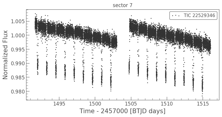
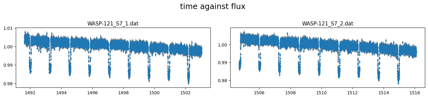
df.scatter()
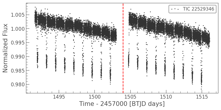
to enable modeling the long-term baseline of the two orbits differently, we can split the orbits.
[5]:
df.split_data(split_times=1504);
Sector 7 data splitted into 2 chunks: ['7_1', '7_2']
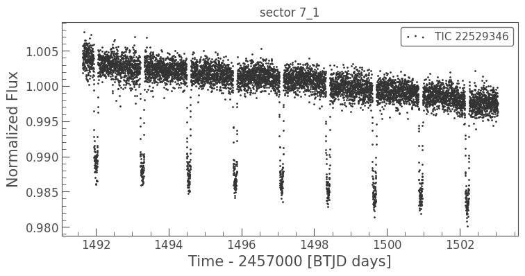
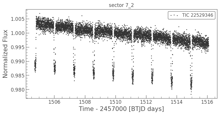
[6]:
df.scatter()
[12]:
df.save_CONAN_lcfile(bjd_ref=2457000)
saved file as: data/WASP-121_S7_1.dat
saved file as: data/WASP-121_S7_2.dat
Data Analysis#
[5]:
from glob import glob
from os.path import basename

import numpy as np
import CONAN
import matplotlib.pyplot as plt
import pandas as pd
CONAN.__version__
[5]:
'3.3.12'
Setup light curve object#
[9]:
path = "data/"
lc_list  = ["WASP-121_S7_1.dat",
            "WASP-121_S7_2.dat",]
[10]:
df = pd.read_fwf(path+lc_list[0], names=[f"col{i}" for i in range(9)])
df.head(5)
[10]:
| col0 | col1 | col2 | col3 | col4 | col5 | col6 | col7 | col8 | |
|---|---|---|---|---|---|---|---|---|---|
| 0 | # time-2457000 flux | flux_err | NaN | NaN | NaN | NaN | NaN | NaN | NaN |
| 1 | 1491.63450126 1.00290573 | 0.00099943 | NaN | NaN | NaN | NaN | NaN | NaN | NaN |
| 2 | 1491.63589017 1.00320482 | 0.00099933 | NaN | NaN | NaN | NaN | NaN | NaN | NaN |
| 3 | 1491.63727908 1.00506699 | 0.00099932 | NaN | NaN | NaN | NaN | NaN | NaN | NaN |
| 4 | 1491.63866798 1.00466049 | 0.00099920 | NaN | NaN | NaN | NaN | NaN | NaN | NaN |
load light curve into CONAN
[11]:
lc_obj = CONAN.load_lightcurves(    file_list     = lc_list,
                                    data_filepath = path,
                                    filters       = ["T"],
                                    wl            = [0.8],
                                    nplanet=1)
lc_obj
# ============ Input lightcurves, filters baseline function =======================================================
name              flt 𝜆_𝜇m |Ssmp ClipOutliers scl_col |off col0 col3 col4 col5 col6 col7 col8|sin id GP spline
WASP-121_S7_1.dat T   0.8  |None None         None    |  y    0    0    0    0    0    0    0|n    1 n  None
WASP-121_S7_2.dat T   0.8  |None None         None    |  y    0    0    0    0    0    0    0|n    2 n  None
[11]:
lightcurves from filepath: data/
1 transiting planet(s)
Order of unique filters: ['T']
The lc_obj object holds information now about the light curves. The light curves can be plotted using the
plotmethod of the object.
By default this plots column 0 (time) against column 1 (flux) with column 3(flux err) as uncertainties.
[12]:
fig = lc_obj.plot(return_fig=True)
[13]:
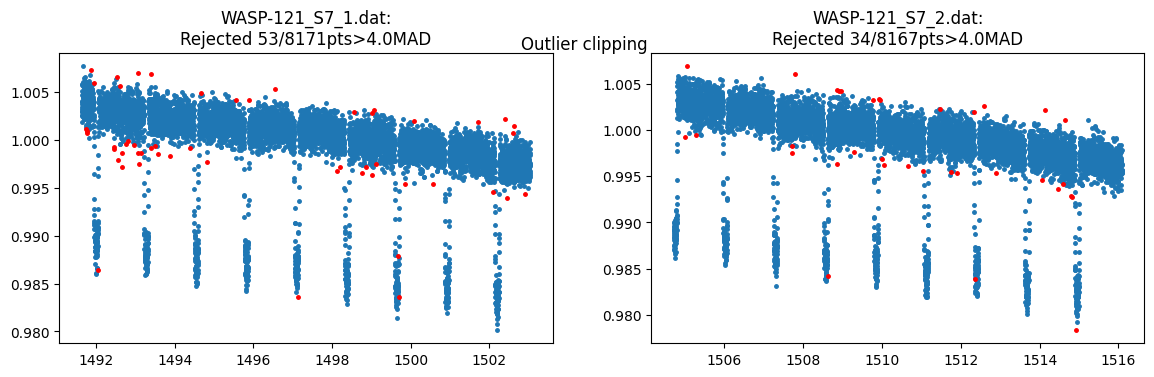
lc_obj.clip_outliers(clip=4, width=15, show_plot=True)
[2]:
from CONAN.get_files import get_parameters
params = get_parameters("WASP-121 b")
params
Loading parameters from cache ...
[2]:
{'star': {'Teff': (6776.0, 138.39),
  'logg': (4.24, 0.01),
  'FeH': (0.13, 0.09),
  'radius': (1.46, 0.03),
  'mass': (1.36, 0.07),
  'density': (0.61186, 0.05357)},
 'planet': {'name': 'WASP-121 b',
  'period': (1.27492504, 1.5e-07),
  'rprs': (0.12355, 0.00033),
  'mass': (1.157, 0.07),
  'ecc': (0.0, nan),
  'w': (10.0, 10.0),
  'T0': (2458119.72074, 0.00017),
  'b': (0.1, 0.01),
  'T14': (0.12105416666666667, 0.0002708333333333333),
  'aR': (nan, nan),
  'K[m/s]': (177.0, 8.5)}}
baseline and decorrelation parameters#
the baseline model for each lightcurve in the lc_obj object can be defined using the
lc_baselinemethodHowever the
get_decorrmethod can be used to automatically determine the best decorrelation parameters to use. (Based on least-squares fit to the data and bayes factor comparison)First, we need to define priors for the planet parameters and limb darkening
[7]:
q1,q2 = lc_obj.get_LDs( Teff        = params["star"]["Teff"],
                        logg        = params["star"]["logg"],
                        Z           = params["star"]["FeH"],
                        filter_names= ["TESS"],
                        unc_mult    = 20)
q1,q2
TESS (T): q1=(0.245, 0.028), q2=(0.3519, 0.0279)
[7]:
([(0.245, 0.028)], [(0.3519, 0.0279)])
[9]:
traocc_pars =dict(  T_0           = (params["planet"]["T0"][0]-2457000,params["planet"]["T0"][1]),
                    Period        = params["planet"]["period"],
                    Impact_para   = (0,params["planet"]["b"][0],0.5),
                    RpRs          = (0.1,params["planet"]["rprs"][0],0.15),
                    Duration      = params["planet"]["T14"],
                    D_occ         = (0,400,600),     #occultation depth in ppm
                    Fn            = (0,10,100),       #Nightside flux in ppm
                    ph_off        = (-7,0,7),       #Phase offset in degrees
                    A_ev          = (0,80,200)        #semi amplitude of ellipsoidal variation in ppm
                    )
The scatter in the differenced lightcurves is used to estimate the level of jitter present in the data and can be accessed using:
[11]:
np.array(lc_obj._jitt_estimate)*1e6 # in ppm
[11]:
array([513.33423946, 634.13728528])
[12]:
decorr_res = lc_obj.get_decorr( **traocc_pars,
                                q1=q1, q2=q2,
                                exclude_cols    = [4,5,6,7,8],
                                use_jitter_est  = True,
                                setup_planet    = True)
getting decorr params for lc01: WASP-121_S7_1.dat (spline=False, sine=False, gp=False, s_samp=False, jitt=513.3ppm)
BEST BIC:8105.54, pars:['offset', 'A0', 'B0']

getting decorr params for lc02: WASP-121_S7_2.dat (spline=False, sine=False, gp=False, s_samp=False, jitt=634.1ppm)
BEST BIC:8012.80, pars:['offset', 'A0']

Setting-up parametric baseline model from decorr result
# ============ Input lightcurves, filters baseline function =======================================================
name              flt 𝜆_𝜇m |Ssmp ClipOutliers scl_col |off col0 col3 col4 col5 col6 col7 col8|sin id GP spline
WASP-121_S7_1.dat T   0.8  |None c1:W15C4n1   None    |  y    2    0    0    0    0    0    0|n    1 n  None
WASP-121_S7_2.dat T   0.8  |None c1:W15C4n1   None    |  y    1    0    0    0    0    0    0|n    2 n  None
Total number of baseline parameters: 5

Setting-up transit pars from input values
# ============ Planet parameters (Transit and RV) setup ==========================================================
name                       fit  prior                                   note
rho_star/[Duration]        y    N(0.12105416666666667,0.0002708333333333333)    #choice in []|unit(gcm^-3/days)
--------repeat this line & params below for multisystem, adding '_planet_number' to the names e.g RpRs_1 for planet 1, ...
RpRs                       y    U(0.1,0.12355,0.15)                     #range[-0.5,0.5]
Impact_para                y    U(0,0.1,0.5)                            #range[0,2]
T_0                        y    N(1119.720739999786,0.00017)            #unit(days)
Period                     y    N(1.27492504,1.5e-07)                   #range[0,inf]days
[Eccentricity]/sesinw      n    F(0)                                    #choice in []|range[0,1]/range[-1,1]
[omega]/secosw             n    F(90)                                   #choice in []|range[0,360]deg/range[-1,1]
K                          n    F(0)                                    #unit(same as RVdata)

Setting-up Phasecurve pars from input values
T: modeling planet's phase_variation with the occultation signal
# ============ Phase curve setup ================================================================================
flt D_occ[ppm]         Fn[ppm]            ph_off[deg]  A_ev[ppm]       f1_ev[ppm]    A_db[ppm]       pc_model
T   U(0,400,600)       U(0,10,100)        U(-7,0,7)    U(0,80,200)     F(0)          F(0)            cosine

Setting-up Limb darkening pars from input values
# ============ Limb darkening setup =============================================================================
filters fit     q1                      q2
T       y       N(0.245,0.028)          N(0.3519,0.0279)
[13]:
decorr_res[0]
[13]:
Fit Result
| fitting method | leastsq |
| # function evals | 217 |
| # data points | 8118 |
| # variables | 14 |
| chi-square | 7979.50941 |
| reduced chi-square | 0.98463838 |
| Akaike info crit. | -113.327136 |
| Bayesian info crit. | 8105.53516 |
| name | value | standard error | relative error | initial value | min | max | vary | expression |
|---|---|---|---|---|---|---|---|---|
| offset | 5.5358e-04 | 4.4433e-05 | (8.03%) | 0 | -0.01985174 | 0.00771880 | True | |
| A0 | -5.1944e-04 | 3.6895e-06 | (0.71%) | 0 | -10.0000000 | 10.0000000 | True | |
| B0 | -1.1234e-05 | 1.2460e-06 | (11.09%) | 0 | -10.0000000 | 10.0000000 | True | |
| A3 | 0.00000000 | 0.00000000 | 0 | -10.0000000 | 10.0000000 | False | ||
| B3 | 0.00000000 | 0.00000000 | 0 | -10.0000000 | 10.0000000 | False | ||
| A4 | 0.00000000 | 0.00000000 | 0 | -10.0000000 | 10.0000000 | False | ||
| B4 | 0.00000000 | 0.00000000 | 0 | -10.0000000 | 10.0000000 | False | ||
| A5 | 0.00000000 | 0.00000000 | 0 | -10.0000000 | 10.0000000 | False | ||
| B5 | 0.00000000 | 0.00000000 | 0 | -10.0000000 | 10.0000000 | False | ||
| A6 | 0.00000000 | 0.00000000 | 0 | -10.0000000 | 10.0000000 | False | ||
| B6 | 0.00000000 | 0.00000000 | 0 | -10.0000000 | 10.0000000 | False | ||
| A7 | 0.00000000 | 0.00000000 | 0 | -10.0000000 | 10.0000000 | False | ||
| B7 | 0.00000000 | 0.00000000 | 0 | -10.0000000 | 10.0000000 | False | ||
| A8 | 0.00000000 | 0.00000000 | 0 | -10.0000000 | 10.0000000 | False | ||
| B8 | 0.00000000 | 0.00000000 | 0 | -10.0000000 | 10.0000000 | False | ||
| T_0 | 1119.72064 | 8.4454e-05 | (0.00%) | 1119.720739999786 | 1119.71904 | 1119.72244 | True | |
| Period | 1.27492502 | 1.4502e-07 | (0.00%) | 1.27492504 | 1.27492354 | 1.27492654 | True | |
| Duration | 0.12079245 | 2.3542e-04 | (0.19%) | 0.12105416666666667 | 0.11834583 | 0.12376250 | True | |
| D_occ | 460.910017 | 55.8469673 | (12.12%) | 400 | 0.00000000 | 600.000000 | True | |
| Impact_para | 0.20303793 | 0.05794368 | (28.54%) | 0.1 | 0.00000000 | 0.50000000 | True | |
| RpRs | 0.11552786 | 4.6387e-04 | (0.40%) | 0.12355 | 0.10000000 | 0.15000000 | True | |
| sesinw | 0.00000000 | 0.00000000 | (nan%) | 0.0 | -inf | inf | False | |
| secosw | 0.00000000 | 0.00000000 | (nan%) | 0.0 | -inf | inf | False | |
| Fn | 83.7669934 | 55.6133719 | (66.39%) | 10 | 0.00000000 | 100.000000 | True | |
| ph_off | -6.99996105 | 14.9593542 | (213.71%) | 0 | -7.00000000 | 7.00000000 | True | |
| A_ev | 7.0989e-05 | 14.0866982 | (19843623.49%) | 80 | 0.00000000 | 200.000000 | True | |
| f1_ev | 0.00000000 | 0.00000000 | 0 | -inf | inf | False | ||
| A_db | 0.00000000 | 0.00000000 | 0 | -inf | inf | False | ||
| q1 | 0.21240451 | 0.01979355 | (9.32%) | 0.245 | 0.00000000 | 1.00000000 | True | |
| q2 | 0.32855395 | 0.02487335 | (7.57%) | 0.3519 | 0.00000000 | 1.00000000 | True | |
| ecc | 0.00000000 | None | 0.00000000 | 1.00000000 | False | sesinw**2+secosw**2 | ||
| w | 0.00000000 | None | 0.00000000 | 360.000000 | False | (180/pi*atan2(sesinw,secosw))%360 | ||
| aR | 3.74568005 | None | 0.00000000 | inf | False | sqrt(((1+abs(RpRs))**2 - Impact_para**2)/(sin( Duration*pi*sqrt(1-ecc**2)/(Period*1**2) )**2 * 1**2)+(Impact_para/1)**2) | ||
| rho_star | 0.61159041 | None | 0.00000000 | inf | False | ((3*pi*aR**3)/((6.674299999999998e-08)*(Period*24*3600)**2))/((1+sqrt(ecc)*sesinw)**3/(1-ecc**2)**(3/2)) | ||
| inc | 86.8927082 | None | -inf | inf | False | (180/pi*acos(Impact_para/(aR*1))) |
| Parameter1 | Parameter 2 | Correlation |
|---|---|---|
| Impact_para | RpRs | +0.7760 |
| offset | D_occ | -0.7277 |
| offset | Fn | -0.7191 |
| D_occ | Fn | +0.7132 |
| RpRs | q1 | -0.7033 |
| Duration | Impact_para | +0.5825 |
| Impact_para | q1 | -0.5195 |
| Fn | A_ev | -0.4719 |
| D_occ | A_ev | -0.4625 |
| q1 | q2 | -0.4133 |
| T_0 | Period | -0.4012 |
| Duration | RpRs | +0.3125 |
| offset | B0 | -0.3062 |
| RpRs | A_ev | -0.1925 |
| RpRs | Fn | +0.1907 |
manually define baseline for each lc
[21]:
# lc_obj.lc_baseline(dcol0=2,gp = "n")
we can include the estimated contamination fraction
[14]:
lc_obj.contamination_factors(cont_ratio=0.0973)
# ============ contamination setup (give contamination as flux ratio) ========================================
flt     contam_factor
T       F(0.0973)
[15]:
lc_obj.print()
# ============ Input lightcurves, filters baseline function =======================================================
name              flt 𝜆_𝜇m |Ssmp ClipOutliers scl_col |off col0 col3 col4 col5 col6 col7 col8|sin id GP spline
WASP-121_S7_1.dat T   0.8  |None c1:W15C4n1   None    |  y    2    0    0    0    0    0    0|n    1 n  None
WASP-121_S7_2.dat T   0.8  |None c1:W15C4n1   None    |  y    1    0    0    0    0    0    0|n    2 n  None
# ============ Sinusoidal signals: Amp*trig(2𝜋/P*(x-x0)) - trig=sin or cos or both added==========================
name/filt         trig     n_harmonics  x     Amp[ppm]            P                   x0
# ============ Photometry GP properties (start newline with name of * or + to Xply or add a 2nd gp to last file) =========
name/filt         kern  par    h1:[Amp]           h2:[len_scale1]    h3:[Q,η,C,α,b]     h4:[P]
# ============ Planet parameters (Transit and RV) setup ==========================================================
name                       fit  prior                                   note
rho_star/[Duration]        y    N(0.12105416666666667,0.0002708333333333333)    #choice in []|unit(gcm^-3/days)
--------repeat this line & params below for multisystem, adding '_planet_number' to the names e.g RpRs_1 for planet 1, ...
RpRs                       y    U(0.1,0.12355,0.15)                     #range[-0.5,0.5]
Impact_para                y    U(0,0.1,0.5)                            #range[0,2]
T_0                        y    N(1119.720739999786,0.00017)            #unit(days)
Period                     y    N(1.27492504,1.5e-07)                   #range[0,inf]days
[Eccentricity]/sesinw      n    F(0)                                    #choice in []|range[0,1]/range[-1,1]
[omega]/secosw             n    F(90)                                   #choice in []|range[0,360]deg/range[-1,1]
K                          n    F(0)                                    #unit(same as RVdata)
# ============ Limb darkening setup =============================================================================
filters fit     q1                      q2
T       y       N(0.245,0.028)          N(0.3519,0.0279)
# ============ ddF setup ========================================================================================
Fit_ddFs        dRpRs                   div_white
n               U(-0.5,0,0.5)           n
# ============ TTV setup ========================================================================================
Fit_TTVs        dt_priors(deviation from linear T0)     transit_baseline[P]     per_LC_T0       include_partial
n               U(-0.125,0,0.125)                                    0.2500     False           True
# ============ Phase curve setup ================================================================================
flt D_occ[ppm]         Fn[ppm]            ph_off[deg]  A_ev[ppm]       f1_ev[ppm]    A_db[ppm]       pc_model
T   U(0,400,600)       U(0,10,100)        U(-7,0,7)    U(0,80,200)     F(0)          F(0)            cosine
# ============ Custom LC function (read from custom_LCfunc.py file)================================================
function        : None                                          #custom function/class to combine with/replace LCmodel
x               : None                                          #independent variable [time, phase_angle]
func_pars       : None                                          #param names&priors e.g. A:U(0,1,2),P:N(2,1)
extra_args      : None                                          #extra args to func as a dict e.g ld_law:quad
op_func         : None                                          #function to combine the LC and custom models
replace_LCmodel : False                                         #if the custom function replaces the LC model
# ============ contamination setup (give contamination as flux ratio) ========================================
flt     contam_factor
T       F(0.0973)
Setup fit#
[16]:
fit_obj = CONAN.fit_setup(  R_st = params['star']['radius'],
                            apply_LCjitter="y",
                            LTT_corr = 'y'  # account for light travel time delay across the orbit
                            )
fit_obj.sampling(n_cpus=10, n_live=150)
# ============ Stellar input properties ======================================================================
# parameter     value
Radius_[Rsun]  N(1.46,0.03)
Mass_[Msun]    N(None,None)
Input_method:[R+rho(Rrho), M+rho(Mrho)]: Rrho
# ============ FIT setup =====================================================================================
Number_steps                              2000
Number_chains                             64
Number_of_processes                       10
Burnin_length                             500
n_live                                    150
force_nlive                               False
d_logz                                    0.1
Sampler(emcee/dynesty)                    dynesty
emcee_move(stretch/demc/snooker)          stretch
nested_sampling(static/dynamic[pfrac])    static
leastsq_for_basepar(y/n)                  n
apply_LCjitter(y/n,list)                  y
apply_RVjitter(y/n,list)                  y
LCjitter_loglims(auto/[lo,hi])            auto
RVjitter_lims(auto/[lo,hi])               auto
LCbasecoeff_lims(auto/[lo,hi])            auto
RVbasecoeff_lims(auto/[lo,hi])            auto
Light_Travel_Time_correction(y/n)         y
apply_LC_GPndim_jitter(y/n)               y
apply_RV_GPndim_jitter(y/n)               y
apply_LC_GPndim_offset(y/n)               y
apply_RV_GPndim_offset(y/n)               y
Save/Load configuration#
we can export the configuration as both a .dat file and a .yaml file.
[17]:
CONAN.create_configfile(lc_obj  = lc_obj,
                        rv_obj  = None,
                        fit_obj = fit_obj,
                        filename='WASP121_TESS_config.dat',
                        verify  = True)
configuration file saved as WASP121_TESS_config.dat
configuration file saved as WASP121_TESS_config.yaml
we can load back either the .dat or .yaml files to obtain the setup again
[6]:
lc_obj, rv_obj, fit_obj = CONAN.load_configfile('WASP121_TESS_config.yaml')
Performing the fit#
we can examine the full set of parameters and priors for the fit
[18]:
CONAN.get_parameter_names(lc_obj, rv_obj, fit_obj)[1]
[18]:
{'Duration': 'N(0.12105416666666667,0.0002708333333333333)',
 'T_0': 'N(1119.720739999786,0.00017)',
 'RpRs': 'U(0.1,0.12355,0.15)',
 'Impact_para': 'U(0,0.1,0.5)',
 'Period': 'N(1.27492504,1.5e-07)',
 'T_DFocc': 'U(0,400,600)',
 'T_Fn': 'U(0,10,100)',
 'T_ph_off': 'U(-7,0,7)',
 'T_Aev': 'U(0,80,200)',
 'T_q1': 'N(0.2450,0.0280)',
 'T_q2': 'N(0.3519,0.0279)',
 'lc1_logjitter': 'U(-15.0000,-7.5746,-4.6390)',
 'lc2_logjitter': 'U(-15.0000,-7.3632,-4.6398)',
 'lc1_off': 'U(0.98014826,1,1.0077188)',
 'lc1_A0': 'U(-1,0,1)',
 'lc1_B0': 'U(-1,0,1)',
 'lc2_off': 'U(0.97918314,1,1.00584662)',
 'lc2_A0': 'U(-1,0,1)'}
Notice that there is a jitter for each lightcurve (lc1_logjitter, lc2_logjitter) as is the default in CONAN. However, since both lightcurves are from same TESS sector, they can share the same jitter.
This can be done by configuring them as shared_params as a dictionary that maps one or several “recipient” parameters to one “donor” parameter in the format: shared_params = { donor : [recipient]}
[19]:
shared_params = {'lc1_logjitter': ['lc2_logjitter']}
we can confirm that lc2_logjitter is no longer a parameter to fit, as it now shares values with lc1_logjitter
[22]:
CONAN.get_parameter_names(lc_obj, rv_obj, fit_obj,shared_params)[1]
[22]:
{'Duration': 'N(0.12105416666666667,0.0002708333333333333)',
 'T_0': 'N(1119.720739999786,0.00017)',
 'RpRs': 'U(0.1,0.12355,0.15)',
 'Impact_para': 'U(0,0.1,0.5)',
 'Period': 'N(1.27492504,1.5e-07)',
 'T_DFocc': 'U(0,400,600)',
 'T_Fn': 'U(0,10,100)',
 'T_ph_off': 'U(-7,0,7)',
 'T_Aev': 'U(0,80,200)',
 'T_q1': 'N(0.2450,0.0280)',
 'T_q2': 'N(0.3519,0.0279)',
 'lc1_logjitter': 'U(-15.0000,-7.5746,-4.6390)',
 'lc1_off': 'U(0.98014826,1,1.0077188)',
 'lc1_A0': 'U(-1,0,1)',
 'lc1_B0': 'U(-1,0,1)',
 'lc2_off': 'U(0.97918314,1,1.00584662)',
 'lc2_A0': 'U(-1,0,1)'}
Finally, we perform the fitting which is saved to a results object that holds the sampling chains and allows subsequent plotting
[23]:
result = CONAN.run_fit( lc_obj  = lc_obj,
                        rv_obj  = rv_obj,
                        fit_obj = fit_obj,
                        shared_params = shared_params,
                        out_folder   = "result_WASP121",
                        rerun_result = True);
Creating output folder...result_WASP121
configuration file saved as result_WASP121/config_save.dat
configuration file saved as result_WASP121/config_save.yaml

================ CONAN fit launched!!! ================

Setting up photometry arrays ...

Plotting prior distributions ...
----------------------------------

Generating initial model(s) ...
--------------------------- [0.78 secs]

Plotting initial model(s) ...
--------------------------- [6.23 secs]

Fit setup
----------
No of cpus: 10
No of dimensions: 17
fitting parameters:  ['Duration' 'T_0' 'RpRs' 'Impact_para' 'Period' 'T_DFocc' 'T_Fn'
 'T_ph_off' 'T_Aev' 'T_q1' 'T_q2' 'lc1_logjitter' 'lc1_off' 'lc1_A0'
 'lc1_B0' 'lc2_off' 'lc2_A0']
Shared parameters:  {'lc1_logjitter': ['lc2_logjitter']}

============ Samping started ... (using dynesty [static])======================
WARNING: Number of dynesty live points is less than 10*ndim. Increasing number of live points to min(10*ndim, 1000)
No of live points:  170
13167it [45:15, 4.85it/s, +170 | bound: 434 | nc: 1 | ncall: 483465 | eff(%): 2.760 | loglstar: -inf < 87460.441 < inf | logz: 87385.489 +/- 0.722 | dlogz: 0.001 > 0.100]
Dynesty chain written to disk as result_WASP121/chains_dict.pkl. Run `result=CONAN.load_result()` to load it.

============ Sampling Finished ==============================================[0.77hrs]

Making corner plot(s) ...
----> saved 2 corner plot(s) as result_WASP121/corner_*.png [9.98 secs]


Creating *out.dat files using the median posterior ...
    - Writing LC output to file: result_WASP121/out_data/WASP-121_S7_1_lcout.dat
    - Writing LC output to file: result_WASP121/out_data/WASP-121_S7_2_lcout.dat

 ----> Plotting figures using median posterior values ...[3.75 secs]

 ----> Plotting figures using max posterior values ...[3.52 secs]

Computing AIC, BIC stats ...[0.00 secs]

Computing photometric noise (red and white) correction factors ... [40.33308386802673 secs


['lc'] Output files, ['WASP-121_S7_1_lcout.dat', 'WASP-121_S7_2_lcout.dat'], loaded into result object
load_lightcurves(): input_lc is provided, using it to load lightcurves.
['rv'] Output files, [], loaded into result object
load_rvs(): input_rv is provided, using it to load rvs.
Linking the last created lightcurve object to the rv object for parameter linking. if this is not the related LC object, input the correct one using `lc_obj` argument of `load_rvs()`
.

CONAN: I have now crushed your data,
        the planetary information it hides is laid bare in the results.
                I am super ready for another quest.
Results#
[ ]:
import CONAN
import matplotlib.pyplot as plt
from CONAN.utils import bin_data, phase_fold
[25]:
result =CONAN.load_result("result_WASP121")
['lc'] Output files, ['WASP-121_S7_1_lcout.dat', 'WASP-121_S7_2_lcout.dat'], loaded into result object
load_lightcurves(): input_lc is provided, using it to load lightcurves.
['rv'] Output files, [], loaded into result object
load_rvs(): input_rv is provided, using it to load rvs.
Linking the last created lightcurve object to the rv object for parameter linking. if this is not the related LC object, input the correct one using `lc_obj` argument of `load_rvs()`
.
[26]:
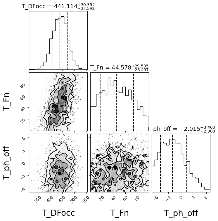
result.plot_corner(['T_DFocc', 'T_Fn', 'T_ph_off']);
[31]:
result.params_dict
[31]:
{'Duration': 0.12096762774345829+/-0.00015973513970569952,
 'T_0': 1119.7206454087868+/-6.678174133867287e-05,
 'RpRs': 0.12130404278518352+/-0.00023892596201999933,
 'Impact_para': 0.07416901671256881+/-0.0465637478339153,
 'Period': 1.2749249737678017+/-1.3548965083209907e-07,
 'T_DFocc': 441.19633269640065+/-31.696721584647378,
 'T_Fn': 44.533002348196014+/-28.35724453775935,
 'T_ph_off': -2.017930514129997+/-3.164099545433184,
 'T_Aev': 5.893275056750161+/-5.98263754405342,
 'T_q1': 0.19241814432464402+/-0.015489750290541754,
 'T_q2': 0.30864992169562017+/-0.0213733497059595,
 'lc1_logjitter': -7.502706188891717+/-0.01943533025929156,
 'lc1_off': 1.000597577832784+/-2.6675177079438228e-05,
 'lc1_A0': -0.0005204066701743892+/-3.1924381915238165e-06,
 'lc1_B0': -1.116321569216705e-05+/-1.2052121489691814e-06,
 'lc2_off': 0.9996200043258529+/-2.3190918743531963e-05,
 'lc2_A0': -0.000605945149427578+/-3.55729308937347e-06}
LC#
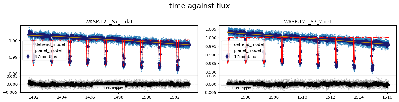
[32]:
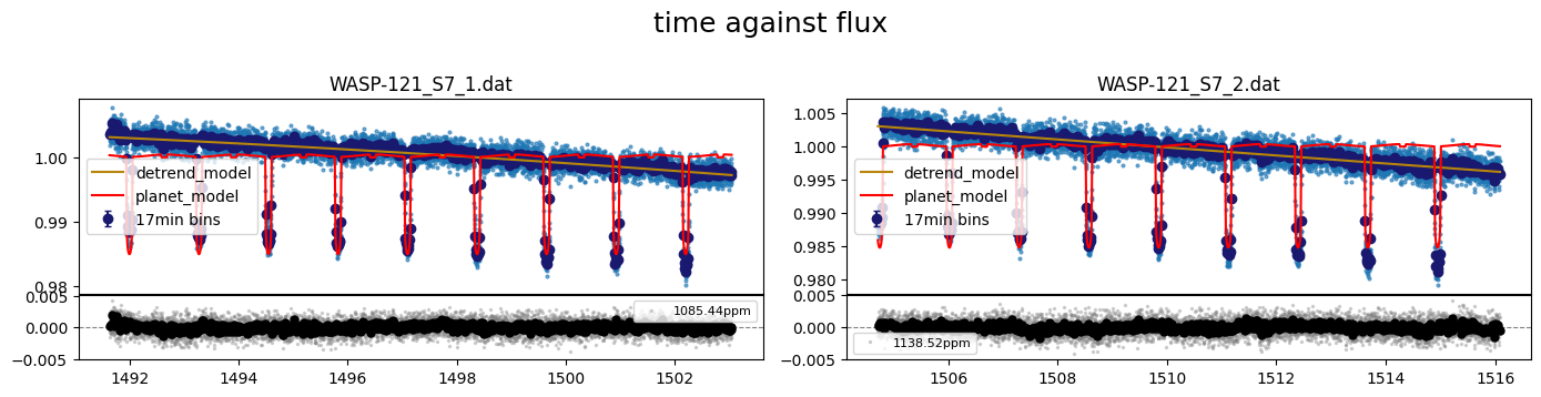
result.lc.plot_bestfit();
[33]:
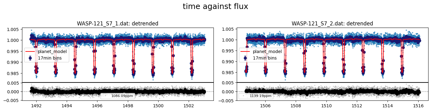
result.lc.plot_bestfit(detrend=True)
[33]:
