WASP-127b: Fitting only RVs#
[1]:
import numpy as np
import CONAN
import matplotlib.pyplot as plt
import pandas as pd
CONAN.__version__
[1]:
'3.3.12'
[ ]:
from CONAN.get_files import get_parameters

sys_params = get_parameters(planet_name="WASP-127b")
sys_params
Setup RV#
The RV setup is similar to the LC
[3]:
path ="../data/"
rv_list = ["rv1.dat","rv2.dat"]    #rv data in km/s
[6]:
rv_obj = CONAN.load_rvs(file_list     = rv_list,
                         data_filepath = path,
                         rv_unit       ='km/s',
                         nplanet       = 1,
                        )
rv_obj
Linking the last created lightcurve object to the rv object for parameter linking. if this is not the related LC object, input the correct one using `lc_obj` argument of `load_rvs()`
.
# ============ Input RV curves, baseline function, GP, spline,  gamma ============================================
name    RVunit scl_col |col0 col3 col4 col5| sin GP spline_config   | gamma_km/s
rv1.dat km/s   None    |   0    0    0    0|   0 n  None            | F(0.0)
rv2.dat km/s   None    |   0    0    0    0|   0 n  None            | F(0.0)
[6]:
rvs from filepath: ../data/
1 planet(s)
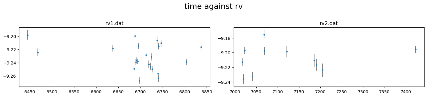
[7]:
rv_obj.plot()
[8]:
rv_obj.rescale_data_columns()
Rescaled data columns of rv1.dat with method:med_sub
Rescaled data columns of rv2.dat with method:med_sub
Baseline and decorrelation#
similar to lightcurves, we can manually specify the rv baseline model using the
.rv_baseline()method
[9]:
rv_obj.rv_baseline( dcol0 = None,
                    dcol3 = None,
                    dcol4 = None,
                    dcol5 = None,
                    gamma = [(-9.232,0.1),    #systemic velocity rv1
                             (-9.21,0.1)],    #systemic velocity rv2
                    )
# ============ Input RV curves, baseline function, GP, spline,  gamma ============================================
name    RVunit scl_col |col0 col3 col4 col5| sin GP spline_config   | gamma_km/s
rv1.dat km/s   med_sub |   0    0    0    0|   0 n  None            | N(-9.232,0.1)
rv2.dat km/s   med_sub |   0    0    0    0|   0 n  None            | N(-9.21,0.1)
or we can use the
.get_decorr()method to find the best decorrelation.
By setting setup_planet=True the planet parameter priors are also passed to the planet_parameters() and we dont need to do that again, unless we wish to change the priors
[10]:
t0  = sys_params["planet"]["T0"][0] - 2450000
P   = sys_params["planet"]["period"][0]

rvdecorr_res= rv_obj.get_decorr(T_0           = t0,     #fixed
                                Period        = P,      #fixed
                                Eccentricity  = 0,
                                omega         = 90,
                                K             = (0,10e-3,100e-3),     #km/s
                                gamma        = (-9.21,0.1),
                                delta_BIC    = -5,
                                setup_planet = True)
getting decorr params for rv01: rv1.dat (jitt=0.00km/s)

BEST BIC:85.63, pars:['B0']

getting decorr params for rv02: rv2.dat (jitt=0.00km/s)

BEST BIC:14.02, pars:[]
Setting-up rv baseline model from result
# ============ Input RV curves, baseline function, GP, spline,  gamma ============================================
name    RVunit scl_col |col0 col3 col4 col5| sin GP spline_config   | gamma_km/s
rv1.dat km/s   med_sub |   2    0    0    0|   0 n  None            | N(-9.233510019201736,0.1)
rv2.dat km/s   med_sub |   0    0    0    0|   0 n  None            | N(-9.210554832954267,0.1)

Setting-up planet RV pars from input values
# ============ Planet parameters (Transit and RV) setup ==========================================================
name                       fit  prior                                   note
[rho_star]/Duration        n    F(0)                                    #choice in []|unit(gcm^-3/days)
--------repeat this line & params below for multisystem, adding '_planet_number' to the names e.g RpRs_1 for planet 1, ...
RpRs                       n    F(0)                                    #range[-0.5,0.5]
Impact_para                n    F(0)                                    #range[0,2]
T_0                        n    F(6776.621239999775)                    #unit(days)
Period                     n    F(4.17806203)                           #range[0,inf]days
[Eccentricity]/sesinw      n    F(0)                                    #choice in []|range[0,1]/range[-1,1]
[omega]/secosw             n    F(90)                                   #choice in []|range[0,360]deg/range[-1,1]
K                          y    U(0,0.01,0.1)                           #unit(same as RVdata)
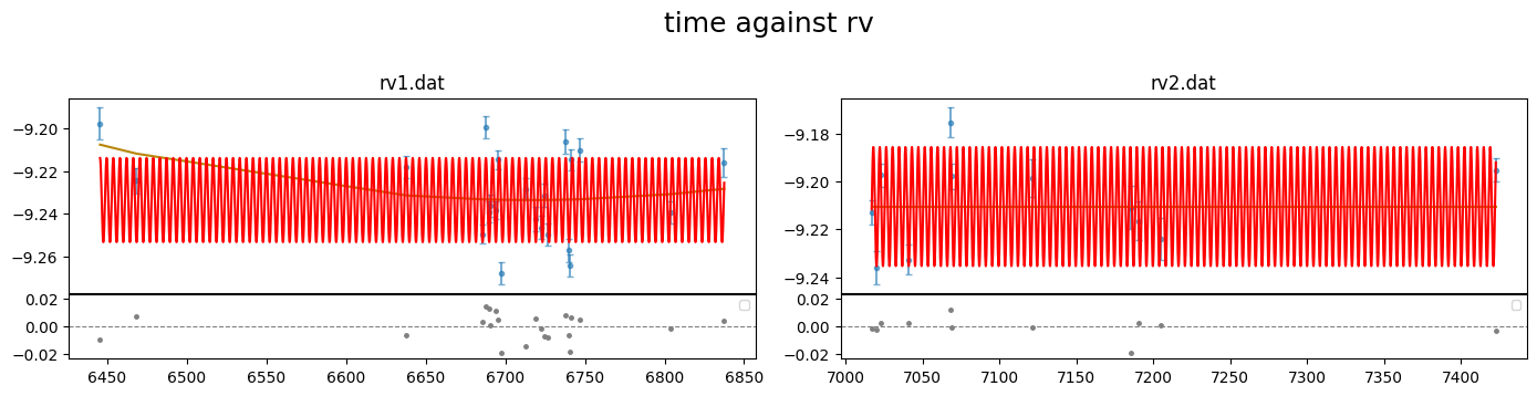
[11]:
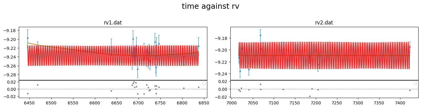
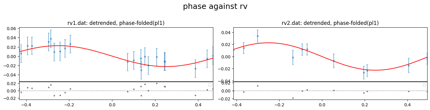
rv_obj.plot(detrend=True, show_decorr_model=True, phase_plot=1)
Setup Sampling#
finally to setup the fit_obj which is used to configure the fitting.
We can specify values for the stellar mass or radius to be used to convert parameter results to physical values. These values are not used in the fit, only for the post-fit conversion. The values from our NASA archive sys_params dictionary
[12]:
sys_params["star"]["radius"], sys_params["star"]["mass"]
[12]:
((1.333, 0.027), (0.95, 0.02))
setup sampling using the .sampling() method of fit_obj. Note that the sampling of the parameter space can be done with emcee or dynesty. The default is dynesty
[4]:
fit_obj = CONAN.fit_setup( M_st = sys_params["star"]["mass"],
                            par_input = "Mrho",
                            apply_RVjitter="y",
                            verbose=False)

fit_obj.sampling(sampler="dynesty",n_cpus=10, n_live=100, verbose=False)
Export configuration#
All configuration can be exported to a config.dat file that allows to reproduce all steps and eventually run the fit
[5]:
CONAN.create_configfile(None, rv_obj, fit_obj,
                         filename='wasp127_rv_config.dat')
configuration file saved as wasp127_rv_config.dat
configuration file saved as wasp127_rv_config.yaml
[3]:
# #reload objects from config file
import CONAN
lc_obj, rv_obj, fit_obj = CONAN.load_configfile('wasp127_rv_config.dat')
load_lightcurves(): loading lightcurves from path -  /Users/tunde/Library/CloudStorage/OneDrive-unige.ch/mygit/CONAN/Notebooks/WASP-127/WASP127_RV/../data/
load_rvs(): loading RVs from path - /Users/tunde/Library/CloudStorage/OneDrive-unige.ch/mygit/CONAN/Notebooks/WASP-127/WASP127_RV/../data/
Sampling#
Finally perform the fitting which returns a result object result_obj that holds the chains of the mcmc and allows subsequent plotting.
The result of the fit is saved to a user-defined folder (default = ‘output’). If a fit result already exists in this folder, it is loaded to the result_obj
[ ]:
result = CONAN.run_fit(lc_obj  = None,
                        rv_obj  = rv_obj,
                        fit_obj = fit_obj,
                        out_folder="result_wasp127_rv_fit",
                        rerun_result=True);
Results#
[17]:
import CONAN
import matplotlib.pyplot as plt
from CONAN.utils import bin_data, phase_fold
[18]:
result =CONAN.load_result(folder="result_wasp127_rv_fit")
result
['lc'] Output files, [], loaded into result object
['rv'] Output files, ['rv1_rvout.dat', 'rv2_rvout.dat'], loaded into result object
[18]:
Object containing posterior from emcee/dynesty sampling
Parameters in chain are:
         ['K', 'rv1_gamma', 'rv1_jitter', 'rv2_gamma', 'rv2_jitter', 'rv1_A0', 'rv1_B0']

use `plot_chains()`, `plot_burnin_chains()`, `plot_corner()` or `plot_posterior()` methods on selected parameters to visualize results.
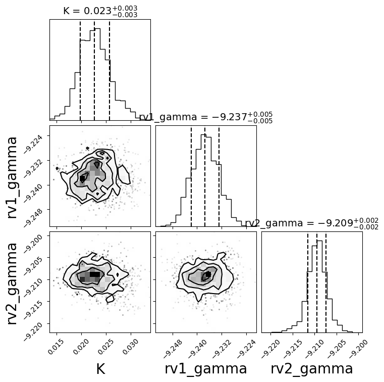
[20]:
fig = result.plot_corner(pars =['K','rv1_gamma','rv2_gamma']);
RVs#
[21]:
result.rv.names
[21]:
['rv1.dat', 'rv2.dat']
[22]:
fig = result.rv.plot_bestfit()
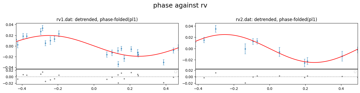
[23]:
result.rv.plot_bestfit(detrend=True, phase_plot=1);
[24]:
#load output data files for the rv fits
rv1data = result.rv.outdata['rv1.dat']
rv2data = result.rv.outdata['rv2.dat']
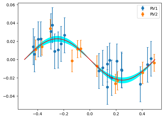
[25]:
#evaluate RV model on a smoother time array
t_sm  = np.linspace(rv1data["time"].min(), rv1data["time"].max(), 1000)
rvmod = result.rv.evaluate(file="rv1.dat",time=t_sm, return_std=True)

phases = phase_fold(t=t_sm, per=result.params.P,
                    t0=result.params.T0, phase0=-0.5)
#sort
srt    = np.argsort(phases)
[26]:
plt.errorbar(rv1data["phase"],rv1data["det_RV"],rv1data["error"],fmt="o",capsize=2,label="RV1")
plt.errorbar(rv2data["phase"],rv2data["det_RV"],rv2data["error"],fmt="o",capsize=2,label="RV2")

plt.plot(phases[srt], rvmod.planet_model[srt],"r",zorder=5)

plt.fill_between(phases[srt],rvmod.sigma_low[srt], rvmod.sigma_high[srt], color="cyan")


plt.legend()
[26]:
<matplotlib.legend.Legend at 0x139233e50>
[ ]: