WASP-127: Fitting multiple LCs#
[3]:
from glob import glob
from os.path import basename

import numpy as np
import CONAN
import matplotlib.pyplot as plt
import pandas as pd
CONAN.__version__
[3]:
'3.3.12'
The CONAN has 3 major classes that are used to store information about the input files and also perform computations.
They are:
load_lightcurves(): ingest lightcurve files and creates an object that is used to configure baseline and model parameters. It contains methods to configure the LCs for fittingload_rvs(): same as above but for rvsfit_setup(): object to setup sampling of the parameter space
These objects are then given as input to the run_fit() function to perform sampling.
Setup light curve object#
[2]:
path = "../data/"    #path to the lightcurve files

lc_list  = sorted(glob(f"{path}*bjd.dat"))   #select euler lightcurves
lc_list = [basename(lc) for lc in lc_list]
lc_list
[2]:
['lc1bjd.dat',
 'lc2bjd.dat',
 'lc3bjd.dat',
 'lc4bjd.dat',
 'lc5bjd.dat',
 'lc6bjd.dat',
 'lc7bjd.dat']
load light curve into CONAN and visualize#
[3]:
lc_obj = CONAN.load_lightcurves( file_list     = lc_list,
                                  data_filepath = path,
                                  filters       = ["R"],
                                  nplanet       = 1)
lc_obj
# ============ Input lightcurves, filters baseline function =======================================================
name       flt 𝜆_𝜇m |Ssmp ClipOutliers scl_col |off col0 col3 col4 col5 col6 col7 col8|sin id GP spline
lc1bjd.dat R   0.6  |None None         None    |  y    0    0    0    0    0    0    0|n    1 n  None
lc2bjd.dat R   0.6  |None None         None    |  y    0    0    0    0    0    0    0|n    2 n  None
lc3bjd.dat R   0.6  |None None         None    |  y    0    0    0    0    0    0    0|n    3 n  None
lc4bjd.dat R   0.6  |None None         None    |  y    0    0    0    0    0    0    0|n    4 n  None
lc5bjd.dat R   0.6  |None None         None    |  y    0    0    0    0    0    0    0|n    5 n  None
lc6bjd.dat R   0.6  |None None         None    |  y    0    0    0    0    0    0    0|n    6 n  None
lc7bjd.dat R   0.6  |None None         None    |  y    0    0    0    0    0    0    0|n    7 n  None
[3]:
lightcurves from filepath: ../data/
1 transiting planet(s)
Order of unique filters: ['R']
The lightcurve object
lc_objholds information about the light curves (data and settings).
By default they are all deactivated. We will define the ones relevant options for this notebook
clip: outlier clipping
scl_col: scaling the arrays in the columns of the data
col{x}: polynomial order in the columns x={0,3,4,5,6,7} of the data to use for decorrelation
Visualizing the data#
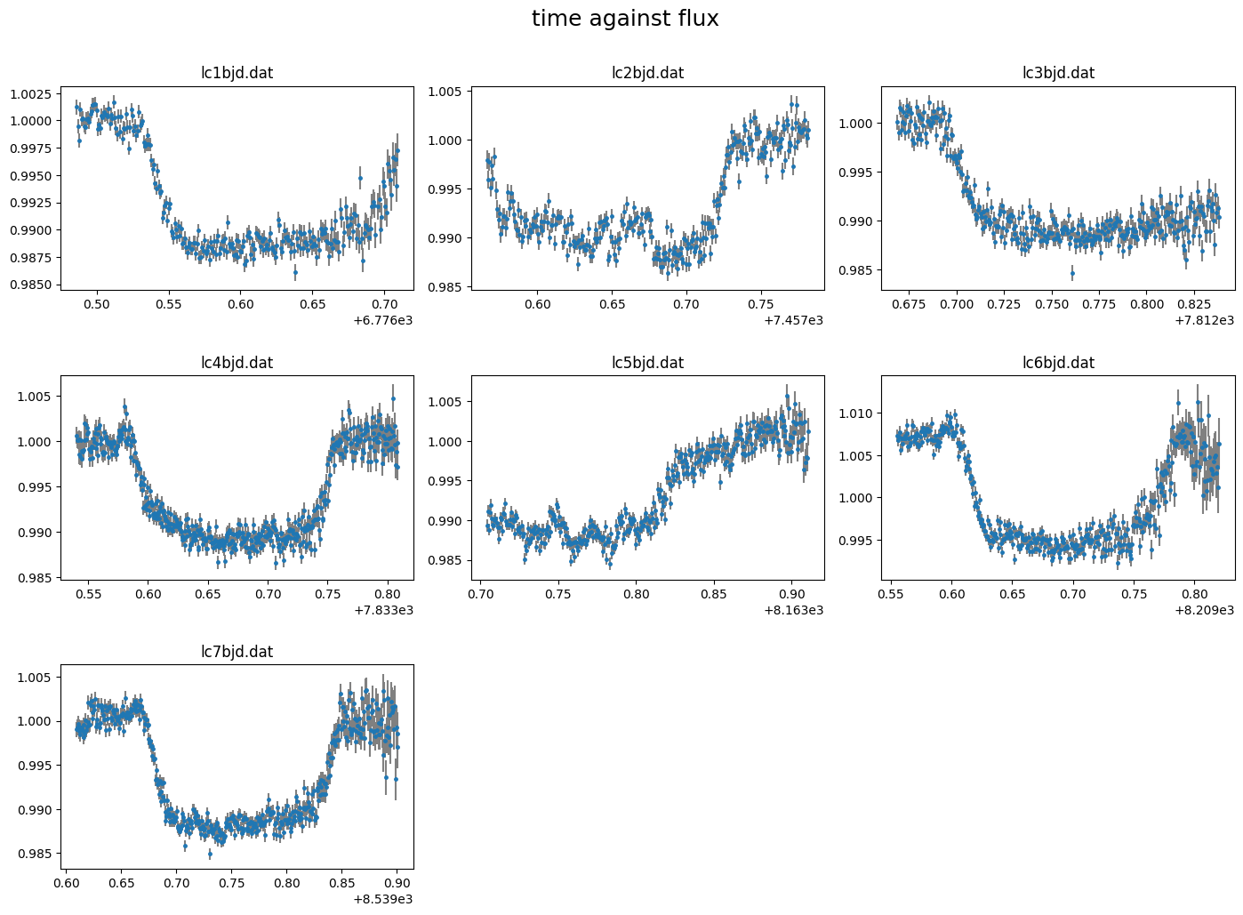
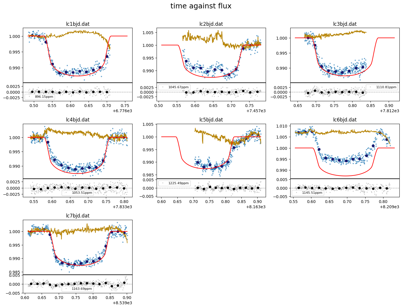
The light curves can be plotted using the plot() method of the object.
By default this plots column 0 (time) against column 1 (flux) with column 3(flux err) as uncertainties.
[4]:
lc_obj.plot()
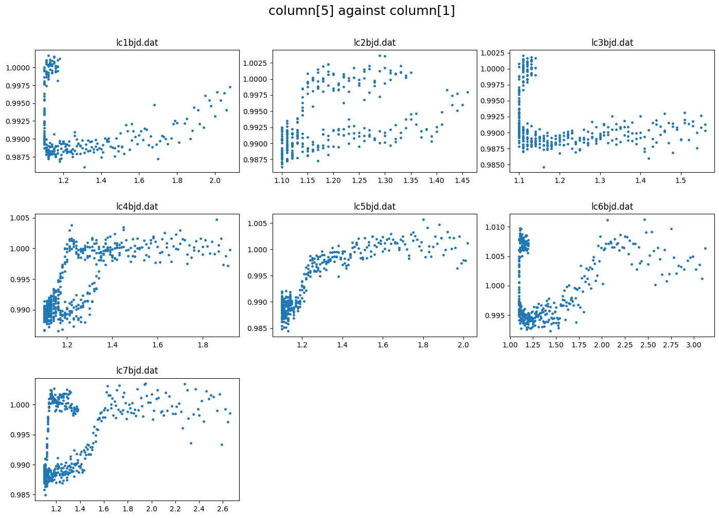
correlations between the flux and other columns in the lightcurve file can be visualized by specifying the columns to plot. e.g. to plot column5 against column 1 (flux)
[5]:
lc_obj.plot(plot_cols=(5,1))
some data processing#
clipping outlier points#
we can remove outliers from all or specific lcs. This uses a sliding median of specified width to discard points greater than clip\(\times\) the M.A.D (median absoulte deviation). The clipped data is saved to the lc_obj further analysis is performed on the clipped data
[ ]:
lc_obj.clip_outliers(lc_list="all", width=11, clip=4)
rescaling data columns.#
This is useful for decorrelating the flux against the different columns. It is only performed on columns 3 and above whose values do not span zero. There are 3 methods to rescale the data: “med_sub”, “rs0to1”, “rs-1to1” which subtracts the median, rescales to [0-1], or rescales to [-1,1] respectively
[7]:
lc_obj.rescale_data_columns(method="med_sub")
Rescaled data columns of lc1bjd.dat with method:med_sub
Rescaled data columns of lc2bjd.dat with method:med_sub
Rescaled data columns of lc3bjd.dat with method:med_sub
Rescaled data columns of lc4bjd.dat with method:med_sub
Rescaled data columns of lc5bjd.dat with method:med_sub
Rescaled data columns of lc6bjd.dat with method:med_sub
Rescaled data columns of lc7bjd.dat with method:med_sub
Setup Transit#
Parameters are defined in CONAN in 3 formats:
Fixed: int/float e.g
q1= 0.5Uniform prior: tuple of length 3 –> (min, start, max) e.g.
Period= (0, 0.5, 1)Normal prior: tuple of length 2 –> (mean, sigma) e.g.
rho_star= (0.5, 0.03)
system parameters#
We can get system parameters from the NASA exoplanet archive
[4]:
from CONAN.get_files import get_parameters

sys_params = get_parameters(planet_name="WASP-127b") #result cached in the current working directory
sys_params
Loading parameters from cache ...
[4]:
{'star': {'Teff': (5620.0, 85.0),
  'logg': (4.18, 0.01),
  'FeH': (-0.193, 0.014),
  'radius': (1.333, 0.027),
  'mass': (0.95, 0.02),
  'density': (0.569, 0.021)},
 'planet': {'name': 'WASP-127 b',
  'period': (4.17806203, 8.8e-07),
  'rprs': (0.10103, 0.00026),
  'mass': (0.1647, 0.0214),
  'ecc': (0.0, nan),
  'w': (nan, nan),
  'T0': (2456776.62124, 0.00023),
  'b': (0.29, 0.04),
  'T14': (0.18137, 0.00035),
  'aR': (7.81, 0.11),
  'K[m/s]': (22.0, 3.0)}}
Transit and RV#
The sys_params can be used to specify the priors for the planet’s transit and RV parameters
Let’s put the planet parameters in a dictionary for convenience. The parameters are defined for transit/occultation/phasecurve/rv
[9]:
t0  = sys_params["planet"]["T0"][0] - 2450000

planet_pars = dict( T_0           = (t0, 0.001),                            # normal prior
                    Period        = sys_params["planet"]["period"][0],      # fixed
                    rho_star      = sys_params["star"]["density"],          # normal pripr
                    Impact_para   = (0, sys_params["planet"]["b"][0], 1),   # uniform prior
                    RpRs          = (0.05, 0.102, 0.17),                    # uniform prior
                    Eccentricity  = 0,                                      # fixed
                    omega         = 90,
                    K             = 0)
The .planet_parameters() method of lc_obj is called to define the parameters in CONAN. This method takes in the same parameter names as defined in planet_pars dictionary so we can load this directly
[10]:
lc_obj.planet_parameters(**planet_pars)
# ============ Planet parameters (Transit and RV) setup ==========================================================
name                       fit  prior                                   note
[rho_star]/Duration        y    N(0.569,0.021)                          #choice in []|unit(gcm^-3/days)
--------repeat this line & params below for multisystem, adding '_planet_number' to the names e.g RpRs_1 for planet 1, ...
RpRs                       y    U(0.05,0.102,0.17)                      #range[-0.5,0.5]
Impact_para                y    U(0,0.29,1)                             #range[0,2]
T_0                        y    N(6776.621239999775,0.001)              #unit(days)
Period                     n    F(4.17806203)                           #range[0,inf]days
[Eccentricity]/sesinw      n    F(0)                                    #choice in []|range[0,1]/range[-1,1]
[omega]/secosw             n    F(90)                                   #choice in []|range[0,360]deg/range[-1,1]
K                          n    F(0)                                    #unit(same as RVdata)
Limb darkening#
The
sys_paramscan also be used to obtain priors on the stellar limb darkening from the phoenix stellar library.CONANuses the Kipping parameterization of the quadratic law defined as \(q_1\) and \(q_2\).
Filter names can be obtained from the SVO filter service with names such as Spitzer/IRAC.I1 or a name shortcut such as TESS, CHEOPS,kepler.
List of filter shortcut names can be obtained using:
[11]:
lc_obj._filter_shortcuts
[11]:
{'kepler': 'Kepler/Kepler.k',
 'tess': 'TESS/TESS.Red',
 'cheops': 'CHEOPS/CHEOPS.band',
 'wfc3_g141': 'HST/WFC3_IR.G141',
 'wfc3_g102': 'HST/WFC3_IR.G102',
 'sp36': 'Spitzer/IRAC.I1',
 'sp45': 'Spitzer/IRAC.I2',
 'ug': 'Geneva/Geneva.U',
 'b1': 'Geneva/Geneva.B1',
 'b2': 'Geneva/Geneva.B2',
 'bg': 'Geneva/Geneva.B',
 'gg': 'Geneva/Geneva.G',
 'v1': 'Geneva/Geneva.V2',
 'vg': 'Geneva/Geneva.V',
 'sdss_g': 'SLOAN/SDSS.g',
 'sdss_r': 'SLOAN/SDSS.r',
 'sdss_i': 'SLOAN/SDSS.i',
 'sdss_z': 'SLOAN/SDSS.z'}
specify a filter for the EULER
[12]:
filts = ['sdss_r']
[13]:
print(f"\nGetting limb darkening parameters for filter {filts}")
q1, q2 = lc_obj.get_LDs( Teff = sys_params['star']['Teff'],
                        logg  = sys_params['star']['logg'],
                        Z     = sys_params['star']['FeH'],
                        filter_names=filts,
                        # fixed_unc=0.02   #use uncertainty of 0.02 for all q1 and q2 values
            )
Getting limb darkening parameters for filter ['sdss_r']
sdss_r    (R): q1=(0.4221, 0.0197), q2=(0.3961, 0.0129)
q1, q2 can then be passed to the .limb_darkening() method of lc_obj
[14]:
lc_obj.limb_darkening(q1=q1, q2=q2)
# ============ Limb darkening setup =============================================================================
filters fit     q1                      q2
R       y       N(0.4221,0.0197)        N(0.3961,0.0129)
Baseline and decorrelation parameters#
The baseline model for each lightcurve in lc_obj object can be defined manually or automagically
Manually define baseline model:#
We manually define the baseline model using the .lc_baseline() method of the lc_obj
Define baseline model parameters to fit for each light curve using the columns of the input data. dcol0 refers to decorrelation setup for column 0, dcol3 for column 3, and so on.
Each baseline decorrelation parameter (dcol{x}) should be a list of integers specifying the polynomial order for column {x} for each light curve. e.g. Given 2 input light curves as we have here,
If one wishes to fit a 1st order trend in column 0 (time) to all lightcurves, then dcol0 = 1. This creates a so we have lc{n}_A0, where {n} goes from 1 to the number of loaded lightcurves, and A0 depicts first order in column 0.
For most of the input lightcurves, we saw a strong correlation of the flux with column 5. We can fit this with a 2nd order term by setting dcol5 = 2. this creates lc{n}_A5 and lc{n}_B5, as second order fit B5 necessarily includes the first oder A5.
[15]:
lc_obj.lc_baseline( dcol0 = 1,
                    dcol5 = 2)
# ============ Input lightcurves, filters baseline function =======================================================
name       flt 𝜆_𝜇m |Ssmp ClipOutliers scl_col |off col0 col3 col4 col5 col6 col7 col8|sin id GP spline
lc1bjd.dat R   0.6  |None c1:W11C4n1   med_sub |  y    1    0    0    2    0    0    0|n    1 n  None
lc2bjd.dat R   0.6  |None c1:W11C4n1   med_sub |  y    1    0    0    2    0    0    0|n    2 n  None
lc3bjd.dat R   0.6  |None c1:W11C4n1   med_sub |  y    1    0    0    2    0    0    0|n    3 n  None
lc4bjd.dat R   0.6  |None c1:W11C4n1   med_sub |  y    1    0    0    2    0    0    0|n    4 n  None
lc5bjd.dat R   0.6  |None c1:W11C4n1   med_sub |  y    1    0    0    2    0    0    0|n    5 n  None
lc6bjd.dat R   0.6  |None c1:W11C4n1   med_sub |  y    1    0    0    2    0    0    0|n    6 n  None
lc7bjd.dat R   0.6  |None c1:W11C4n1   med_sub |  y    1    0    0    2    0    0    0|n    7 n  None
There’s no guarantee this is the optimal baseline model. The .get_decorr() function of the lc_obj can be used to automatically determine the best decorrelation parameters to use.
To do this, we would like take into account the transit/occultation when peforming the least-squares fit. So the defined transit parameter priors in planet_pars are also used
[16]:
decorr_res = lc_obj.get_decorr( **planet_pars,
                                q1 = q1,    q2 = q2,
                                delta_BIC      = -5,
                                exclude_cols   = [8], #exclude this column(exptime)
                                setup_baseline = True
                                )
getting decorr params for lc01: lc1bjd.dat (spline=False, sine=False, gp=False, s_samp=False, jitt=0.0ppm)
BEST BIC:378.98, pars:['offset', 'A6', 'A4']

getting decorr params for lc02: lc2bjd.dat (spline=False, sine=False, gp=False, s_samp=False, jitt=0.0ppm)
BEST BIC:549.14, pars:['offset', 'A6', 'A0', 'B7']

getting decorr params for lc03: lc3bjd.dat (spline=False, sine=False, gp=False, s_samp=False, jitt=0.0ppm)
BEST BIC:562.80, pars:['offset', 'A6', 'A7']

getting decorr params for lc04: lc4bjd.dat (spline=False, sine=False, gp=False, s_samp=False, jitt=0.0ppm)
BEST BIC:706.68, pars:['offset', 'A6']

getting decorr params for lc05: lc5bjd.dat (spline=False, sine=False, gp=False, s_samp=False, jitt=0.0ppm)
BEST BIC:756.34, pars:['offset', 'B0', 'A6', 'B3', 'B5']

getting decorr params for lc06: lc6bjd.dat (spline=False, sine=False, gp=False, s_samp=False, jitt=0.0ppm)
BEST BIC:678.02, pars:['offset', 'A6', 'B5', 'A5']

getting decorr params for lc07: lc7bjd.dat (spline=False, sine=False, gp=False, s_samp=False, jitt=0.0ppm)
BEST BIC:590.81, pars:['offset', 'A6', 'B5']

Setting-up parametric baseline model from decorr result
# ============ Input lightcurves, filters baseline function =======================================================
name       flt 𝜆_𝜇m |Ssmp ClipOutliers scl_col |off col0 col3 col4 col5 col6 col7 col8|sin id GP spline
lc1bjd.dat R   0.6  |None c1:W11C4n1   med_sub |  y    0    0    1    0    1    0    0|n    1 n  None
lc2bjd.dat R   0.6  |None c1:W11C4n1   med_sub |  y    1    0    0    0    1    2    0|n    2 n  None
lc3bjd.dat R   0.6  |None c1:W11C4n1   med_sub |  y    0    0    0    0    1    1    0|n    3 n  None
lc4bjd.dat R   0.6  |None c1:W11C4n1   med_sub |  y    0    0    0    0    1    0    0|n    4 n  None
lc5bjd.dat R   0.6  |None c1:W11C4n1   med_sub |  y    2    2    0    2    1    0    0|n    5 n  None
lc6bjd.dat R   0.6  |None c1:W11C4n1   med_sub |  y    0    0    0    2    1    0    0|n    6 n  None
lc7bjd.dat R   0.6  |None c1:W11C4n1   med_sub |  y    0    0    0    2    1    0    0|n    7 n  None
Total number of baseline parameters: 29
the output decorr_res is a list that holds the lmfit result for each lc.
By specifying use_result=True in the function call above, several other lightcurve configuration (baseline, gp, transit&RV parameters, phase curve, limb darkening) that uses the same inputs have been automatically set up
We can use the .plot() method again to visualize the fit quality across the different decorrelation axis by setting show_decorr_model=True
[17]:
lc_obj.plot(plot_cols=(5,1), show_decorr_model=True)

We can use the .print() method to print out the current configuration of the different sections of the lc_obj
To see the current baseline model configuration, set section to “lc_baseline”
[18]:
lc_obj.print(section="lc_baseline")
# ============ Input lightcurves, filters baseline function =======================================================
name       flt 𝜆_𝜇m |Ssmp ClipOutliers scl_col |off col0 col3 col4 col5 col6 col7 col8|sin id GP spline
lc1bjd.dat R   0.6  |None c1:W11C4n1   med_sub |  y    0    0    1    0    1    0    0|n    1 n  None
lc2bjd.dat R   0.6  |None c1:W11C4n1   med_sub |  y    1    0    0    0    1    2    0|n    2 n  None
lc3bjd.dat R   0.6  |None c1:W11C4n1   med_sub |  y    0    0    0    0    1    1    0|n    3 n  None
lc4bjd.dat R   0.6  |None c1:W11C4n1   med_sub |  y    0    0    0    0    1    0    0|n    4 n  None
lc5bjd.dat R   0.6  |None c1:W11C4n1   med_sub |  y    2    2    0    2    1    0    0|n    5 n  None
lc6bjd.dat R   0.6  |None c1:W11C4n1   med_sub |  y    0    0    0    2    1    0    0|n    6 n  None
lc7bjd.dat R   0.6  |None c1:W11C4n1   med_sub |  y    0    0    0    2    1    0    0|n    7 n  None
Setup Sampling#
finally to setup the fit_obj which is used to configure the fitting.
We can specify values for the stellar mass or radius to be used to convert parameter results to physical values. These values are not used in the fit, only for the post-fit conversion. We can also take the values from our NASA archive sys_params dictionary
[19]:
sys_params["star"]["radius"], sys_params["star"]["mass"]
[19]:
((1.333, 0.027), (0.95, 0.02))
[5]:
fit_obj = CONAN.fit_setup(  R_st      = sys_params["star"]["radius"],
                            M_st      = sys_params["star"]["mass"],
                            par_input = "Rrho",
                          )
# ============ Stellar input properties ======================================================================
# parameter     value
Radius_[Rsun]  N(1.333,0.027)
Mass_[Msun]    N(0.95,0.02)
Input_method:[R+rho(Rrho), M+rho(Mrho)]: Rrho
setup sampling using the .sampling() method of fit_obj. Note that the sampling of the parameter space can be done with emcee or dynesty
[6]:
fit_obj.sampling(sampler="dynesty",n_cpus = 10, n_live=300)
# ============ FIT setup =====================================================================================
Number_steps                              2000
Number_chains                             64
Number_of_processes                       10
Burnin_length                             500
n_live                                    300
force_nlive                               False
d_logz                                    0.1
Sampler(emcee/dynesty)                    dynesty
emcee_move(stretch/demc/snooker)          stretch
nested_sampling(static/dynamic[pfrac])    static
leastsq_for_basepar(y/n)                  n
apply_LCjitter(y/n,list)                  y
apply_RVjitter(y/n,list)                  y
LCjitter_loglims(auto/[lo,hi])            auto
RVjitter_lims(auto/[lo,hi])               auto
LCbasecoeff_lims(auto/[lo,hi])            auto
RVbasecoeff_lims(auto/[lo,hi])            auto
Light_Travel_Time_correction(y/n)         n
apply_LC_GPndim_jitter(y/n)               y
apply_RV_GPndim_jitter(y/n)               y
apply_LC_GPndim_offset(y/n)               y
apply_RV_GPndim_offset(y/n)               y
export configuration file#
[ ]:
CONAN.create_configfile(lc_obj  = lc_obj,
                         rv_obj  = None,
                         fit_obj = fit_obj,
                         filename='wasp127_euler_config.dat')
load_rvs(): loading RVs from path - /Users/tunde/Library/CloudStorage/OneDrive-unige.ch/mygit/CONAN/Notebooks/WASP-127/WASP-127_EULER_LC/
Linking the last created lightcurve object to the rv object for parameter linking. if this is not the related LC object, input the correct one using `lc_obj` argument of `load_rvs()`
.
configuration file saved as wasp127_euler_config.dat
[1]:
import CONAN
lc_obj, rv_obj, fit_obj = CONAN.load_configfile(configfile='wasp127_euler_config.dat')
load_lightcurves(): loading lightcurves from path -  /Users/tunde/Library/CloudStorage/OneDrive-unige.ch/mygit/CONAN/Notebooks/WASP-127/WASP-127_EULER_LC/../data/
load_rvs(): loading RVs from path - /Users/tunde/Library/CloudStorage/OneDrive-unige.ch/mygit/CONAN/Notebooks/WASP-127/WASP-127_EULER_LC/
Sampling#
Finally perform the fitting which returns a result object result_obj that holds the chains from the sampling and allows subsequent plotting.
The result of the fit is saved to a user-defined folder (default = ‘output’). If a fit result already exists in this folder, it is loaded to the result_obj
[ ]:
result = CONAN.run_fit(lc_obj  = lc_obj,
                        rv_obj  = None,
                        fit_obj = fit_obj,
                        out_folder="result_wasp127_euler",
                        rerun_result=True);
The summary statistics of the fitted and derived parameters are written as **result_*.dat** files in the output folder.
results#
[1]:
import CONAN
import matplotlib.pyplot as plt
import numpy as np
from CONAN.utils import bin_data, phase_fold
[4]:
result =CONAN.load_result(folder="result_wasp127_euler")
['lc'] Output files, ['lc1bjd_lcout.dat', 'lc2bjd_lcout.dat', 'lc3bjd_lcout.dat', 'lc4bjd_lcout.dat', 'lc5bjd_lcout.dat', 'lc6bjd_lcout.dat', 'lc7bjd_lcout.dat'], loaded into result object
['rv'] Output files, [], loaded into result object
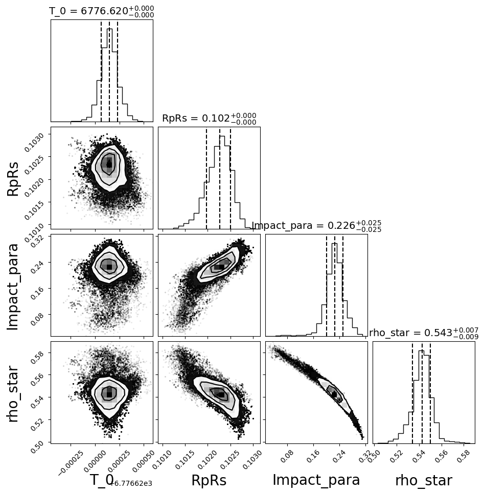
[5]:
fig = result.plot_corner(pars = ['T_0', 'RpRs', 'Impact_para', 'rho_star']);
make output file for max posterior values#
the output files are generated from the median posterior values. The user can create output models from the maximum posterior
[6]:
result.make_output_file("max",
                        out_folder="result_wasp127_euler/max_out_data")
    - Writing LC output to file: result_wasp127_euler/max_out_data/out_data/lc1bjd_lcout.dat
    - Writing LC output to file: result_wasp127_euler/max_out_data/out_data/lc2bjd_lcout.dat
    - Writing LC output to file: result_wasp127_euler/max_out_data/out_data/lc3bjd_lcout.dat
    - Writing LC output to file: result_wasp127_euler/max_out_data/out_data/lc4bjd_lcout.dat
    - Writing LC output to file: result_wasp127_euler/max_out_data/out_data/lc5bjd_lcout.dat
    - Writing LC output to file: result_wasp127_euler/max_out_data/out_data/lc6bjd_lcout.dat
    - Writing LC output to file: result_wasp127_euler/max_out_data/out_data/lc7bjd_lcout.dat
LC#
[7]:
result.lc.names
[7]:
['lc1bjd.dat',
 'lc2bjd.dat',
 'lc3bjd.dat',
 'lc4bjd.dat',
 'lc5bjd.dat',
 'lc6bjd.dat',
 'lc7bjd.dat']
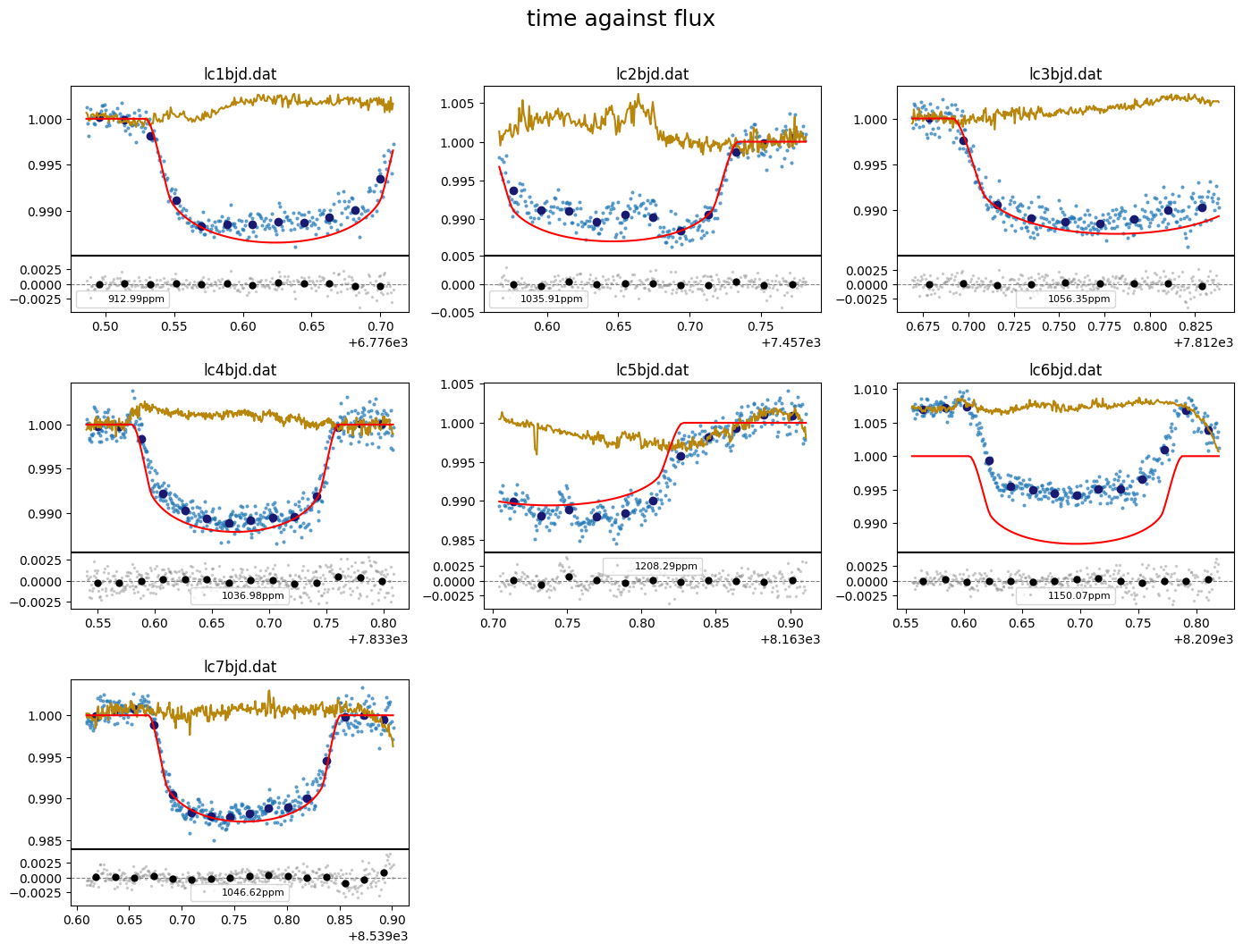
[9]:
fig = result.lc.plot_bestfit()
make plots from results#
[10]:
import pandas as pd
# concatenate output of all LCs
lc_data = pd.concat([result.lc.outdata[nm] for nm in result.lc.outdata.keys()])
[11]:
#evaluate LC model on a different time array
t_sm  = np.linspace(lc_data["time"].min(), lc_data["time"].max()+0.02, 3000)

lcmod  = result.lc.evaluate(time=t_sm, return_std=True)

phases = phase_fold(t=t_sm, per=result.params.P,
                    t0=result.params.T0, phase0=-0.5)
#sort
srt    = np.argsort(phases)
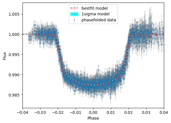
[12]:
plt.errorbar(lc_data["phase"],lc_data["det_flux"],lc_data["error"],
             fmt="o",ms=3,ecolor="gray",alpha=0.3,capsize=2,label="phasefolded data")

plt.plot(phases[srt], lcmod.planet_model[srt],"r--",zorder=4, label="bestfit model")
plt.fill_between(phases[srt],lcmod.sigma_low[srt], lcmod.sigma_high[srt], color="cyan",
                 zorder=3,label="1sigma model")

plt.xlabel("Phase")
plt.ylabel("Flux")
plt.xlim([-0.04,0.04])
plt.legend();
[ ]:
[ ]:
[ ]: