WASP-103b: 2D GP with George#

Data Analysis#

[1]:

from glob import glob
import numpy as np
import CONAN
import matplotlib.pyplot as plt

from os.path import basename
import pandas as pd
CONAN.__version__

[1]:

'3.3.12'

[2]:

from CONAN.get_files import get_parameters
P          = 0.925545485
BJD_0      =  2457511.944458 -2457000
sys_params = get_parameters("WASP-103")
path       = "data/"

Loading parameters from cache ...

In order to derive different occultation depths for the observations, we will set different filters

[3]:

lc_obj = CONAN.load_lightcurves(
                                file_list       = 'WASP-103_000905.dat',
                                data_filepath   = path,
                                filters         = "CH",
                                wl              = 0.6)

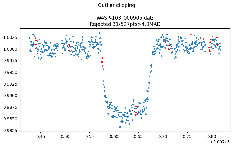
lc_obj.clip_outliers(   width   = 15,
                        clip    = 4,
                        select_column =  ["col1","col6"],
                        niter       = 1,
                        show_plot   = True,
                        verbose     = False)

../_images/tutorial_WASP-103_2D-GP-george_5_0.png

[4]:

lc_obj.rescale_data_columns(columns=[3,4,6,7,8],verbose=False)

[5]:

q1 = (0.4287, 0.0666)
q2 = (0.4023, 0.0284)

[6]:

t14 = sys_params['planet']['T14'][0]
tra_occ_pars =dict( T_0         = (BJD_0-0.1,BJD_0,BJD_0+0.1),
                    Period      = (P,5e-8),
                    Impact_para = (0,0.1,1),
                    RpRs        = (0.09,0.113,0.13),
                    Duration    = (0.8*t14, t14, 1.2*t14))
tra_occ_pars

[6]:

{'T_0': (511.84445799989624, 511.94445799989626, 512.0444579998963),
 'Period': (0.925545485, 5e-08),
 'Impact_para': (0, 0.1, 1),
 'RpRs': (0.09, 0.113, 0.13),
 'Duration': (0.08643333333333333, 0.10804166666666666, 0.12965)}

[7]:

lc_obj.add_GP(  lc_list     = "all",
                par         = ("col5",     "col8"),
                kernel      = ( "mat32",    "mat32"),
                operation   = "+",
                amplitude   = ( (1,200, 1000), (1,200,1000) ),
                lengthscale = ((0.1, 10, 50),  (0.01, 0.5, 1.5) ),
                gp_pck      = "ge"
            )

# ============ Input lightcurves, filters baseline function =======================================================
name                flt 𝜆_𝜇m |Ssmp ClipOutliers scl_col |off col0 col3 col4 col5 col6 col7 col8|sin id GP spline
WASP-103_000905.dat CH  0.6  |None c16:W15C4n1  med_sub |  n    0    0    0    0    0    0    0|n    1 ge None
# ============ Photometry GP properties (start newline with name of * or + to Xply or add a 2nd gp to last file) =========
name/filt           kern  par    h1:[Amp]           h2:[len_scale1]    h3:[Q,η,C,α,b]     h4:[P]
all                 mat32 col5   U(1,200,1000)      U(0.1,10,50)       None               None
                |+| mat32 col8   U(1,200,1000)      U(0.01,0.5,1.5)    None               None

Least squares fit#

Let’s do a least squares fit with this setup

[8]:

decorr_res = lc_obj.get_decorr(
                                **tra_occ_pars,
                                q1              = q1,
                                q2              = q2,
                                delta_BIC       = -5,
                                exclude_cols    = [0,3,4,5,6,7,8],
                                setup_planet    = True,
                                show_steps      = False,
                                use_jitter_est  = False,
                                cont            = 0.092)


getting decorr params for lc01: WASP-103_000905.dat (spline=False, sine=False, gp=True, s_samp=False, jitt=0.0ppm)
BEST BIC:484.62, pars:[]

Setting-up parametric baseline model from decorr result
# ============ Input lightcurves, filters baseline function =======================================================
name                flt 𝜆_𝜇m |Ssmp ClipOutliers scl_col |off col0 col3 col4 col5 col6 col7 col8|sin id GP spline
WASP-103_000905.dat CH  0.6  |None c16:W15C4n1  med_sub |  n    0    0    0    0    0    0    0|n    1 ge None
Total number of baseline parameters: 0

Setting-up transit pars from input values
# ============ Planet parameters (Transit and RV) setup ==========================================================
name                       fit  prior                                   note
rho_star/[Duration]        y    U(0.08643333333333333,0.10804166666666666,0.12965)      #choice in []|unit(gcm^-3/days)
--------repeat this line & params below for multisystem, adding '_planet_number' to the names e.g RpRs_1 for planet 1, ...
RpRs                       y    U(0.09,0.113,0.13)                      #range[-0.5,0.5]
Impact_para                y    U(0,0.1,1)                              #range[0,2]
T_0                        y    U(511.84445799989624,511.94445799989626,512.0444579998963)      #unit(days)
Period                     y    N(0.925545485,5e-08)                    #range[0,inf]days
[Eccentricity]/sesinw      n    F(0)                                    #choice in []|range[0,1]/range[-1,1]
[omega]/secosw             n    F(90)                                   #choice in []|range[0,360]deg/range[-1,1]
K                          n    F(0)                                    #unit(same as RVdata)

Setting-up Phasecurve pars from input values
CH: modeling only occultation signal
# ============ Phase curve setup ================================================================================
flt D_occ[ppm]         Fn[ppm]            ph_off[deg]  A_ev[ppm]       f1_ev[ppm]    A_db[ppm]       pc_model
CH  F(0)               None               None         F(0)            F(0)          F(0)            cosine

Setting-up Limb darkening pars from input values
# ============ Limb darkening setup =============================================================================
filters fit     q1                      q2
CH      y       N(0.4287,0.0666)        N(0.4023,0.0284)

../_images/tutorial_WASP-103_2D-GP-george_11_1.png

[9]:

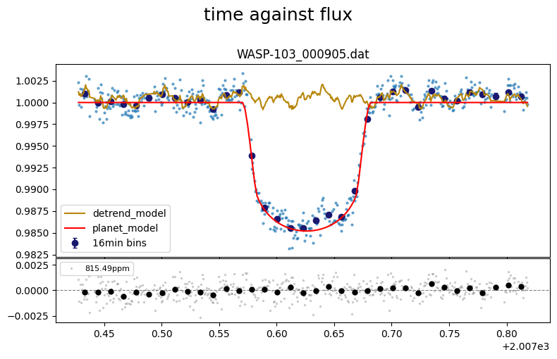
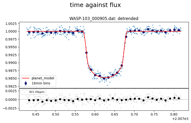
lc_obj.plot(show_decorr_model=True, detrend=True, phase_plot=0)

../_images/tutorial_WASP-103_2D-GP-george_12_0.png

[10]:

decorr_res[0]

[10]:

Fit Result

Fit Statistics
fitting method	L-BFGS-B
# function evals	1944
# data points	496
# variables	11
chi-square	416.352208
reduced chi-square	0.85845816
Akaike info crit.	128.842758
Bayesian info crit.	484.624543

Parameters
name	value	initial value	min	max	vary	expression
offset	0.00000000	0	-0.01677698	0.00338933	False
A0	0.00000000	0	-10.0000000	10.0000000	False
B0	0.00000000	0	-10.0000000	10.0000000	False
A3	0.00000000	0	-10.0000000	10.0000000	False
B3	0.00000000	0	-10.0000000	10.0000000	False
A4	0.00000000	0	-10.0000000	10.0000000	False
B4	0.00000000	0	-10.0000000	10.0000000	False
A5	0.00000000	0	-10.0000000	10.0000000	False
B5	0.00000000	0	-10.0000000	10.0000000	False
A6	0.00000000	0	-10.0000000	10.0000000	False
B6	0.00000000	0	-10.0000000	10.0000000	False
A7	0.00000000	0	-10.0000000	10.0000000	False
B7	0.00000000	0	-10.0000000	10.0000000	False
A8	0.00000000	0	-10.0000000	10.0000000	False
B8	0.00000000	0	-10.0000000	10.0000000	False
log_GP_amp1	6.58654937	5.298317366548036	0.00000000	6.90775528	True
log_GP_len1	2.99484666	2.302585092994046	-2.30258509	3.91202301	True
log_GP_h31	-inf	-inf	-inf	inf	False
log_GP_h41	-inf	-inf	-inf	inf	False
log_GP_amp2	5.82598155	5.298317366548036	0.00000000	6.90775528	True
log_GP_len2	-0.69490713	-0.6931471805599453	-4.60517019	0.40546511	True
log_GP_h32	-inf	-inf	-inf	inf	False
log_GP_h42	-inf	-inf	-inf	inf	False
T_0	511.944495	511.94445799989626	511.844458	512.044458	True
Period	0.92554548	0.925545485	0.92554499	0.92554598	True
Duration	0.11072839	0.10804166666666666	0.08643333	0.12965000	True
D_occ	0.00000000	0	-inf	inf	False
Impact_para	0.08728263	0.1	0.00000000	1.00000000	True
RpRs	0.11621747	0.113	0.09000000	0.13000000	True
sesinw	0.00000000	0.0	-inf	inf	False
secosw	0.00000000	0.0	-inf	inf	False
Fn	0.00000000	0	-inf	inf	False
ph_off	0.00000000	0	-inf	inf	False
A_ev	0.00000000	0	-inf	inf	False
f1_ev	0.00000000	0	-inf	inf	False
A_db	0.00000000	0	-inf	inf	False
q1	0.31513981	0.4287	0.00000000	1.00000000	True
q2	0.39107143	0.4023	0.00000000	1.00000000	True
ecc	0.00000000	None	0.00000000	1.00000000	False	sesinw2+secosw2
w	0.00000000	None	0.00000000	360.000000	False	(180/pi*atan2(sesinw,secosw))%360
aR	3.03290788	None	0.00000000	inf	False	sqrt(((1+abs(RpRs))2 - Impact_para2)/(sin( Durationpisqrt(1-ecc*2)/(Period12) )2 * 12)+(Impact_para/1)2)
rho_star	0.61605579	None	0.00000000	inf	False	((3piaR*3)/((6.674299999999998e-08)(Period243600)*2))/((1+sqrt(ecc)sesinw)3/(1-ecc2)**(3/2))
inc	88.3508840	None	-inf	inf	False	(180/piacos(Impact_para/(aR1)))
GP_amp1	725.273895	None	1.00000000	1000.00000	False	exp(log_GP_amp1)
GP_len1	19.9822955	None	0.10000000	50.0000000	False	exp(log_GP_len1)
GP_h31	0.00000000	None	0.00000000	inf	False	exp(log_GP_h31)
GP_h41	0.00000000	None	0.00000000	inf	False	exp(log_GP_h41)
GP_amp2	338.993710	None	1.00000000	1000.00000	False	exp(log_GP_amp2)
GP_len2	0.49912080	None	0.01000000	1.50000000	False	exp(log_GP_len2)
GP_h32	0.00000000	None	0.00000000	inf	False	exp(log_GP_h32)
GP_h42	0.00000000	None	0.00000000	inf	False	exp(log_GP_h42)

Let’s plot the residual of this least-square fit

[11]:

lc_obj.plot((0,"res"), show_decorr_model=True)

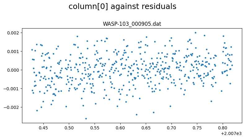
../_images/tutorial_WASP-103_2D-GP-george_15_0.png

Show the correlation of the flux with column 5

[12]:

lc_obj.plot((5,1),show_decorr_model=True, detrend=False, binsize=16/(24*60), phase_plot=0)

../_images/tutorial_WASP-103_2D-GP-george_17_0.png

setup fit#

[13]:

fit_obj = CONAN.fit_setup(  R_st = sys_params["star"]["radius"],
                            M_st = sys_params["star"]["mass"],
                            apply_LCjitter = "y")

fit_obj.sampling(sampler="dynesty",n_cpus=10,n_live=300)

# ============ Stellar input properties ======================================================================
# parameter     value
Radius_[Rsun]  N(1.436,0.052)
Mass_[Msun]    N(1.22,0.039)
Input_method:[R+rho(Rrho), M+rho(Mrho)]: Rrho
# ============ FIT setup =====================================================================================
Number_steps                              2000
Number_chains                             64
Number_of_processes                       10
Burnin_length                             500
n_live                                    300
force_nlive                               False
d_logz                                    0.1
Sampler(emcee/dynesty)                    dynesty
emcee_move(stretch/demc/snooker)          stretch
nested_sampling(static/dynamic[pfrac])    static
leastsq_for_basepar(y/n)                  n
apply_LCjitter(y/n,list)                  y
apply_RVjitter(y/n,list)                  y
LCjitter_loglims(auto/[lo,hi])            auto
RVjitter_lims(auto/[lo,hi])               auto
LCbasecoeff_lims(auto/[lo,hi])            auto
RVbasecoeff_lims(auto/[lo,hi])            auto
Light_Travel_Time_correction(y/n)         n
apply_LC_GPndim_jitter(y/n)               y
apply_RV_GPndim_jitter(y/n)               y
apply_LC_GPndim_offset(y/n)               y
apply_RV_GPndim_offset(y/n)               y

[14]:

fit_obj.print()

# ============ FIT setup =====================================================================================
Number_steps                              2000
Number_chains                             64
Number_of_processes                       10
Burnin_length                             500
n_live                                    300
force_nlive                               False
d_logz                                    0.1
Sampler(emcee/dynesty)                    dynesty
emcee_move(stretch/demc/snooker)          stretch
nested_sampling(static/dynamic[pfrac])    static
leastsq_for_basepar(y/n)                  n
apply_LCjitter(y/n,list)                  y
apply_RVjitter(y/n,list)                  y
LCjitter_loglims(auto/[lo,hi])            auto
RVjitter_lims(auto/[lo,hi])               auto
LCbasecoeff_lims(auto/[lo,hi])            auto
RVbasecoeff_lims(auto/[lo,hi])            auto
Light_Travel_Time_correction(y/n)         n
apply_LC_GPndim_jitter(y/n)               y
apply_RV_GPndim_jitter(y/n)               y
apply_LC_GPndim_offset(y/n)               y
apply_RV_GPndim_offset(y/n)               y

Save and load config file#

[15]:

CONAN.create_configfile(lc_obj,None,fit_obj,filename="WASP103_CHEOPS_2D_GP_george.dat")

configuration file saved as WASP103_CHEOPS_2D_GP_george.dat
configuration file saved as WASP103_CHEOPS_2D_GP_george.yaml

[16]:

import CONAN
lc_obj,rv_obj,fit_obj = CONAN.load_configfile("WASP103_CHEOPS_2D_GP_george.dat")

[ ]:

# ============ Input lightcurves, filters baseline function =======================================================
name                flt 𝜆_𝜇m |Ssmp ClipOutliers scl_col |off col0 col3 col4 col5 col6 col7 col8|sin id GP spline
WASP-103_000905.dat CH  0.6  |None c16:W15C4n1  med_sub |  n    0    0    0    0    0    0    0|n    1 ge None

lightcurves from filepath: data/
1 transiting planet(s)
Order of unique filters: ['CH']

[3]:

fit_obj.print()

# ============ FIT setup =====================================================================================
Number_steps                              2000
Number_chains                             64
Number_of_processes                       10
Burnin_length                             500
n_live                                    300
force_nlive                               False
d_logz                                    0.1
Sampler(emcee/dynesty)                    dynesty
emcee_move(stretch/demc/snooker)          stretch
nested_sampling(static/dynamic[pfrac])    static
leastsq_for_basepar(y/n)                  n
apply_LCjitter(y/n,list)                  y
apply_RVjitter(y/n,list)                  y
LCjitter_loglims(auto/[lo,hi])            auto
RVjitter_lims(auto/[lo,hi])               auto
LCbasecoeff_lims(auto/[lo,hi])            auto
RVbasecoeff_lims(auto/[lo,hi])            auto
Light_Travel_Time_correction(y/n)         n
apply_LC_GPndim_jitter(y/n)               y
apply_RV_GPndim_jitter(y/n)               y
apply_LC_GPndim_offset(y/n)               y
apply_RV_GPndim_offset(y/n)               y

[2]:

CONAN.get_parameter_names(lc_obj,None,fit_obj)[1]

[2]:

{'Duration': 'U(0.08643333333333333,0.10804166666666666,0.12965)',
 'T_0': 'U(511.84445799989624,511.94445799989626,512.0444579998963)',
 'RpRs': 'U(0.09,0.113,0.13)',
 'Impact_para': 'U(0,0.1,1)',
 'Period': 'N(0.925545485,5e-08)',
 'CH_q1': 'N(0.4287,0.0666)',
 'CH_q2': 'N(0.4023,0.0284)',
 'lc1_logjitter': 'U(-15.0000,-8.3116,-4.7217)',
 'GPlc1_Amp1_col5': 'U(1,200,1000)',
 'GPlc1_len1_col5': 'U(0.1,10,50)',
 'GPlc1_Amp2_col8': 'U(1,200,1000)',
 'GPlc1_len2_col8': 'U(0.01,0.5,1.5)'}

Run fit#

[3]:

result = CONAN.run_fit(lc_obj, None, fit_obj,
                        out_folder="result_WASP103_CHEOPS_2D_GP_george",
                        rerun_result=True
                        )

Fit result already exists in this folder: result_WASP103_CHEOPS_2D_GP_george
Rerunning CONAN with saved posterior chains to regenerate plots and files...

load_rvs(): loading RVs from path - /Users/tunde/Library/CloudStorage/OneDrive-unige.ch/mygit/CONAN/Notebooks/WASP-103/
Linking the last created lightcurve object to the rv object for parameter linking. if this is not the related LC object, input the correct one using `lc_obj` argument of `load_rvs()`
.
configuration file saved as result_WASP103_CHEOPS_2D_GP_george/config_save.dat

================ CONAN fit launched!!! ================

Setting up photometry arrays ...
Setting up photometry GPs ...

Plotting prior distributions ...
----------------------------------

Generating initial model(s) ...
--------------------------- [0.04 secs]

Plotting initial model(s) ...
--------------------------- [1.74 secs]

Fit setup
----------
No of cpus: 10
No of dimensions: 12
fitting parameters:  ['Duration' 'T_0' 'RpRs' 'Impact_para' 'Period' 'CH_q1' 'CH_q2'
 'lc1_logjitter' 'GPlc1_Amp1_col5' 'GPlc1_len1_col5' 'GPlc1_Amp2_col8'
 'GPlc1_len2_col8']

============ Samping started ... (using dynesty [static])======================

Skipping dynesty run. Loading chains from disk
============ Sampling Finished ==============================================[0.00hrs]

Making corner plot(s) ...
----> saved 1 corner plot(s) as result_WASP103_CHEOPS_2D_GP_george/corner_*.png [10.20 secs]


Creating *out.dat files using the median posterior ...
    - Writing LC output with GP(George) to file: result_WASP103_CHEOPS_2D_GP_george/out_data/WASP-103_000905_lcout.dat

 ----> Plotting figures using median posterior values ...[1.65 secs]

 ----> Plotting figures using max posterior values ...[1.60 secs]

Computing AIC, BIC stats ...[0.00 secs]

Computing photometric noise (red and white) correction factors ... [0.3004570007324219 secs


['lc'] Output files, ['WASP-103_000905_lcout.dat'], loaded into result object
load_lightcurves(): input_lc is provided, using it to load lightcurves.
['rv'] Output files, [], loaded into result object
load_rvs(): input_rv is provided, using it to load rvs.
Linking the last created lightcurve object to the rv object for parameter linking. if this is not the related LC object, input the correct one using `lc_obj` argument of `load_rvs()`
.

CONAN: I have now crushed your data,
        the planetary information it hides is laid bare in the results.
                I am super ready for another quest.

load result#

[4]:

import CONAN
import matplotlib
import matplotlib.pyplot as plt
%matplotlib inline
import numpy as np

result = CONAN.load_result("result_WASP103_CHEOPS_2D_GP_george")

['lc'] Output files, ['WASP-103_000905_lcout.dat'], loaded into result object
load_lightcurves(): input_lc is provided, using it to load lightcurves.
['rv'] Output files, [], loaded into result object
load_rvs(): input_rv is provided, using it to load rvs.
Linking the last created lightcurve object to the rv object for parameter linking. if this is not the related LC object, input the correct one using `lc_obj` argument of `load_rvs()`
.

[8]:

result.lc.GP['WASP-103_000905.dat'].gp.get_parameter_dict()

[8]:

OrderedDict([('kernel:k1:k1:log_constant', -15.234139330127007),
             ('kernel:k1:k2:metric:log_M_0_0', 5.200939977834735),
             ('kernel:k2:k1:log_constant', -14.751195369171885),
             ('kernel:k2:k2:metric:log_M_0_0', -0.709930881935139)])

We can check if there are still any correlations between the residuals and the cotrending vectors

[2]:

res_corr = result.lc.check_corr(fit_offset="n", delta_BIC=-5)


getting decorr params for lc01: WASP-103_000905.dat (spline=False, sine=False, gp=False, s_samp=False, jitt=0.0ppm)
BEST BIC:486.78, pars:[]

Setting-up parametric baseline model from decorr result
# ============ Input lightcurves, filters baseline function =======================================================
name                flt 𝜆_𝜇m |Ssmp ClipOutliers scl_col |off col0 col3 col4 col5 col6 col7 col8|sin id GP spline
WASP-103_000905.dat CH  0.6  |None None         None    |  n    0    0    0    0    0    0    0|n    1 n  None
Total number of baseline parameters: 0

../_images/tutorial_WASP-103_2D-GP-george_34_1.png

There are no significant correlations left in the residuals

[3]:

result.params_dict

[3]:

{'Duration': 0.11060603470398254+/-0.0006743160444396615,
 'T_0': 511.94453591002923+/-0.00019900574702091944,
 'RpRs': 0.11207642131163673+/-0.0008564380472150523,
 'Impact_para': 0.16771550675584992+/-0.09480373932366967,
 'Period': 0.925545482881369+/-4.946725468135682e-08,
 'CH_q1': 0.30519902052649717+/-0.04223350213719179,
 'CH_q2': 0.38898839647580125+/-0.02810766157423364,
 'lc1_logjitter': -11.264657396739938+/-2.5888577264314225,
 'GPlc1_Amp1_col5': 490.73321723901597+/-97.90373773435346,
 'GPlc1_len1_col5': 13.47017310532421+/-4.973540986210983,
 'GPlc1_Amp2_col8': 626.5796060863466+/-246.43390182281112,
 'GPlc1_len2_col8': 0.7059849988220878+/-0.38741658900076964}

[4]:

result.plot_corner();

../_images/tutorial_WASP-103_2D-GP-george_37_0.png

[6]:

result.lc.plot_bestfit();

../_images/tutorial_WASP-103_2D-GP-george_38_0.png

[7]:

result.lc.plot_bestfit(detrend=True);

../_images/tutorial_WASP-103_2D-GP-george_39_0.png

The GP object is stored in

[14]:

result.lc.GP['WASP-103_000905.dat']

[14]:

GPSaveObj(WASP-103_000905.dat: kernel=['ge_mat32', 'ge_mat32'], ndim=2, cols=('col5', 'col8'), cols_err=None)

[ ]:

WASP-103b: 2D GP with George

Contents