TOI-469: Multiplanet system with LC and RV#
We will analyse the photometry and RV data of the 3-planet system, TOI-469 as published in Damasso et al. 2023
Download data#
[ ]:
from CONAN.get_files import get_TESS_data

df = get_TESS_data("TOI-469")
df.search()
SearchResult containing 11 data products.

 #     mission     year       author      exptime target_name distance
                                             s                 arcsec
--- -------------- ---- ----------------- ------- ----------- --------
  0 TESS Sector 06 2018              SPOC     120    33692729      0.0
  1 TESS Sector 33 2020              SPOC     120    33692729      0.0
  2 TESS Sector 06 2018         TESS-SPOC    1800    33692729      0.0
  3 TESS Sector 33 2020         TESS-SPOC     600    33692729      0.0
  4 TESS Sector 06 2018               QLP    1800    33692729      0.0
  5 TESS Sector 33 2020               QLP     600    33692729      0.0
  6 TESS Sector 06 2018             TASOC     120    33692729      0.0
  7 TESS Sector 06 2018 GSFC-ELEANOR-LITE    1800    33692729      0.0
  8 TESS Sector 06 2018             TASOC    1800    33692729      0.0
  9 TESS Sector 06 2018             TASOC    1800    33692729      0.0
 10 TESS Sector 06 2018              TGLC    1800    33692729      0.0
[3]:
df.download(sectors=[6,33],author="SPOC", select_flux="pdcsap_flux",
            quality_bitmask='default')
downloaded lightcurve for sector 6
downloaded lightcurve for sector 33
[ ]:
df.scatter()
[ ]:
df.lc[6]
[6]:
df.save_CONAN_lcfile(bjd_ref = 2457000, folder="data")
saved file as: data/TOI-469_S6.dat
saved file as: data/TOI-469_S33.dat
Data Analysis#
[1]:
import numpy as np
import matplotlib.pyplot as plt

import CONAN
print(f"CONAN version: {CONAN.__version__}")
CONAN version: 3.3.12
Transit Photometry: 2 sectors of TESS
RV: ESPRESSO
Setup LC object#
[2]:
path = "data/"
lc_list  = ["TOI-469_S06.dat","TOI-469_S33.dat"]
load light curve into CONAN#
[3]:
lc_obj = CONAN.load_lightcurves(file_list      = lc_list,
                                  data_filepath = path,
                                  filters       = ["T"],
                                  lamdas        = [0.8],
                                  nplanet=3)
lc_obj
load_lightcurves(): loading lightcurves from path -  data/
# ============ Input lightcurves, filters baseline function =======================================================
name            flt 𝜆_𝜇m |Ssmp ClipOutliers scl_col |off col0 col3 col4 col5 col6 col7 col8|sin id GP spline
TOI-469_S06.dat T   0.8  |None None         None    |  y    0    0    0    0    0    0    0|n    1 n  None
TOI-469_S33.dat T   0.8  |None None         None    |  y    0    0    0    0    0    0    0|n    2 n  None
[3]:
lightcurves from filepath: data/
3 transiting planet(s)
Order of unique filters: ['T']
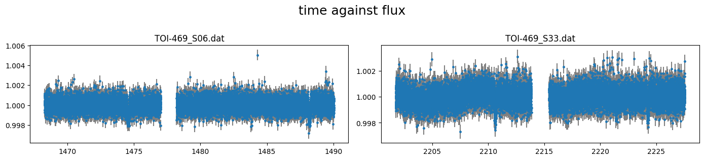
The lc_obj object holds information now about the light curves. The light curves can be plotted using the
plotmethod of the object.
By default this plots column 0 (time) against column 1 (flux) with column 3(flux err) as uncertainties.
[4]:
%matplotlib inline
[5]:
lc_obj.plot()
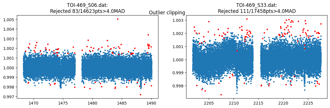
[6]:
lc_obj.clip_outliers(clip=4, width=15, niter=1, show_plot=True)
Planet parameters#
[7]:
traocc_pars =dict( T_0            = [(2210.4,2210.634,2210.8),    #planet 1
                                     (2207.1,2207.252,2207.5),    #planet 2
                                     (2225.1,2225.259,2225.5)],   #planet 3

                    Period        = [(13.6,13.63,13.7),
                                     (3.5,3.5379,3.6),
                                     (6.4,6.42975,6.5)],

                    Impact_para   = [(0, 0.28, 1),
                                     (0, 0.617,1),
                                     (0,0.273,1)],

                    RpRs          = [(0.001,0.0321,0.1),
                                     (0.001,0.0146,0.1),
                                     (0.001,0.0127,0.1)],

                    rho_star      = (1.42,0.1),     #same for all planets

                    K             = (0,2,10)        #m/s - unit of rv data
                  )
[8]:
lc_obj.planet_parameters(**traocc_pars)
# ============ Planet parameters (Transit and RV) setup ==========================================================
name                       fit  prior                                   note
[rho_star]/Duration        y    N(1.42,0.1)                             #choice in []|unit(gcm^-3/days)
--------repeat this line & params below for multisystem, adding '_planet_number' to the names e.g RpRs_1 for planet 1, ...
RpRs_1                     y    U(0.001,0.0321,0.1)                     #range[-0.5,0.5]
Impact_para_1              y    U(0,0.28,1)                             #range[0,2]
T_0_1                      y    U(2210.4,2210.634,2210.8)               #unit(days)
Period_1                   y    U(13.6,13.63,13.7)                      #range[0,inf]days
[Eccentricity_1]/sesinw_1  n    F(0)                                    #choice in []|range[0,1]/range[-1,1]
[omega_1]/secosw_1         n    F(90)                                   #choice in []|range[0,360]deg/range[-1,1]
K_1                        y    U(0,2,10)                               #unit(same as RVdata)
------------
RpRs_2                     y    U(0.001,0.0146,0.1)                     #range[-0.5,0.5]
Impact_para_2              y    U(0,0.617,1)                            #range[0,2]
T_0_2                      y    U(2207.1,2207.252,2207.5)               #unit(days)
Period_2                   y    U(3.5,3.5379,3.6)                       #range[0,inf]days
[Eccentricity_2]/sesinw_2  n    F(0)                                    #choice in []|range[0,1]/range[-1,1]
[omega_2]/secosw_2         n    F(90)                                   #choice in []|range[0,360]deg/range[-1,1]
K_2                        y    U(0,2,10)                               #unit(same as RVdata)
------------
RpRs_3                     y    U(0.001,0.0127,0.1)                     #range[-0.5,0.5]
Impact_para_3              y    U(0,0.273,1)                            #range[0,2]
T_0_3                      y    U(2225.1,2225.259,2225.5)               #unit(days)
Period_3                   y    U(6.4,6.42975,6.5)                      #range[0,inf]days
[Eccentricity_3]/sesinw_3  n    F(0)                                    #choice in []|range[0,1]/range[-1,1]
[omega_3]/secosw_3         n    F(90)                                   #choice in []|range[0,360]deg/range[-1,1]
K_3                        y    U(0,2,10)                               #unit(same as RVdata)
limb darkening#
[9]:
q1,q2 = lc_obj.get_LDs(Teff           = (5289,69),
                       logg           = (4.24,0.13),
                       Z              = (0.24,0.05),
                       filter_names   = ["TESS"],
                       use_result     = True)

# lc_obj.limb_darkening(q1=q1,q2=q2)
TESS      (T): q1=(0.3532, 0.0153), q2=(0.4032, 0.0118)

Setting-up limb-darkening priors from LDTk result
# ============ Limb darkening setup =============================================================================
filters fit     q1                      q2
T       y       N(0.3532,0.0153)        N(0.4032,0.0118)
add GP#
model GP as the only baseline model
get estimate rms of each light curve to use as starting point of gp amplitude
[10]:
np.array(lc_obj._rms_estimate)*1e6
[10]:
array([548.33239097, 571.47486101])
[11]:
lc_obj.add_GP(lc_list     = "all",
              par         = ["col0","col0"],
              kernel      = "mat32",
              amplitude   = (1,100, 700),    #in ppm, uses log-uniform prior
              lengthscale = (0.1,1, 20),    #in days, also log-uniform prior
              gp_pck      = "ce"
             )
# ============ Input lightcurves, filters baseline function =======================================================
name            flt 𝜆_𝜇m |Ssmp ClipOutliers scl_col |off col0 col3 col4 col5 col6 col7 col8|sin id GP spline
TOI-469_S06.dat T   0.8  |None c1:W15C4n1   None    |  n    0    0    0    0    0    0    0|n    1 ce None
TOI-469_S33.dat T   0.8  |None c1:W15C4n1   None    |  n    0    0    0    0    0    0    0|n    2 ce None
# ============ Photometry GP properties (start newline with name of * or + to Xply or add a 2nd gp to last file) =========
name/filt       kern  par    h1:[Amp]           h2:[len_scale1]    h3:[Q,η,C,α,b]     h4:[P]
all             mat32 col0   U(1,100,700)       U(0.1,1,20)        None               None
Setup RV#
[12]:
import CONAN
import matplotlib.pyplot as plt
path = "data/"
[13]:
rv_list = ["TOI469rv1.dat", "TOI469rv2.dat" ]
rv_obj = CONAN.load_rvs(file_list     = rv_list,
                         data_filepath = path,
                         nplanet       = 3,
                         rv_unit       = "m/s",
                         lc_obj        = lc_obj
                        )
rv_obj
load_rvs(): loading RVs from path - data/
# ============ Input RV curves, baseline function, GP, spline,  gamma ============================================
name          RVunit scl_col |col0 col3 col4 col5| sin GP spline_config   | gamma_m/s
TOI469rv1.dat m/s    None    |   0    0    0    0|   0 n  None            | F(0.0)
TOI469rv2.dat m/s    None    |   0    0    0    0|   0 n  None            | F(0.0)
[13]:
rvs from filepath: data/
3 planet(s)
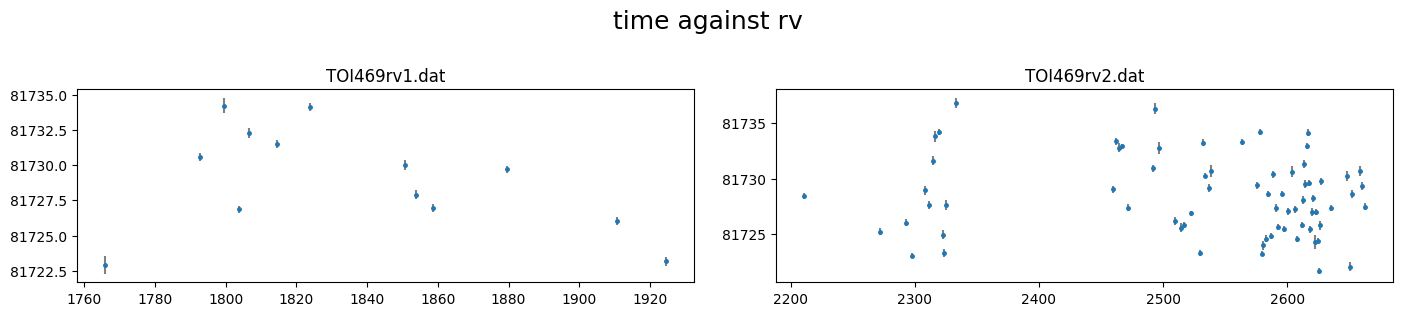
[14]:
rv_obj.plot()
[15]:
rv_obj.rv_baseline(gamma = (81728,10))
# ============ Input RV curves, baseline function, GP, spline,  gamma ============================================
name          RVunit scl_col |col0 col3 col4 col5| sin GP spline_config   | gamma_m/s
TOI469rv1.dat m/s    None    |   0    0    0    0|   0 n  None            | N(81728,10)
TOI469rv2.dat m/s    None    |   0    0    0    0|   0 n  None            | N(81728,10)
add RV GP#
Damasso et al. used a quasiperiodic kernel in time to model stellar activity. We will multiply the exopnential-square (expsq) with a cosine (cos) kernel to acheive the quasiperiodic behaviour.
Note that mutlipling 2 kernels requires the ampltidue of the 2nd kernel to be turned off by setting it to -1
[16]:
rv_obj.add_rvGP(rv_list   = 'same',
              par         = [("col0",        "col0")],
              kernel      = [("cos",         "expsq")],
              amplitude   = [((0.1, 2, 20),    -1)],    #in same unit as rv, uses log-uniform prior
              lengthscale = [((0.01,1, 100), (0.01,1, 60))],    #in days, also log-uniform prior
              operation   = ["*"],
              gp_pck      = "ge"
             )
# ============ Input RV curves, baseline function, GP, spline,  gamma ============================================
name          RVunit scl_col |col0 col3 col4 col5| sin GP spline_config   | gamma_m/s
TOI469rv1.dat m/s    None    |   0    0    0    0|   0 ge None            | N(81728,10)
TOI469rv2.dat m/s    None    |   0    0    0    0|   0 ge None            | N(81728,10)
# ============ RV GP properties (start newline with name of * or + to Xply or add a 2nd gp to last file) =======
name          kern  par    h1:[Amp_ppm]       h2:[len_scale]     h3:[Q,η,C,α,b]     h4:[P]       | h5:[Der_Amp_ppm] ErrCol
same          cos   col0   U(0.1,2,20)        U(0.01,1,100)      None               None         | None             col2
          |*| expsq col0   F(-1)              U(0.01,1,60)       None               None         | None             col2
Setup Sampling#
[17]:
fit_obj = CONAN.fit_setup( R_st = (0.993,0.034),
                            M_st = (0.88,0.035))

fit_obj.sampling(n_cpus=10,n_live=1000)
# ============ Stellar input properties ======================================================================
# parameter     value
Radius_[Rsun]  N(0.993,0.034)
Mass_[Msun]    N(0.88,0.035)
Input_method:[R+rho(Rrho), M+rho(Mrho)]: Rrho
# ============ FIT setup =====================================================================================
Number_steps                              2000
Number_chains                             64
Number_of_processes                       10
Burnin_length                             500
n_live                                    1000
force_nlive                               False
d_logz                                    0.1
Sampler(emcee/dynesty)                    dynesty
emcee_move(stretch/demc/snooker)          stretch
nested_sampling(static/dynamic[pfrac])    static
leastsq_for_basepar(y/n)                  n
apply_LCjitter(y/n,list)                  y
apply_RVjitter(y/n,list)                  y
LCjitter_loglims(auto/[lo,hi])            auto
RVjitter_lims(auto/[lo,hi])               auto
LCbasecoeff_lims(auto/[lo,hi])            auto
RVbasecoeff_lims(auto/[lo,hi])            auto
Light_Travel_Time_correction(y/n)         n
apply_LC_GPndim_jitter(y/n)               y
apply_RV_GPndim_jitter(y/n)               y
apply_LC_GPndim_offset(y/n)               y
apply_RV_GPndim_offset(y/n)               y
Export configuration#
[18]:
CONAN.create_configfile(lc_obj, rv_obj, fit_obj,
                         filename='TOI469_lc_rvconfig.dat')
configuration file saved as TOI469_lc_rvconfig.dat
The config file can be reloaded to create all required objects to perform the fit
[1]:
import CONAN
lc_obj, rv_obj, fit_obj = CONAN.load_configfile('TOI469_lc_rvconfig.dat')
load_lightcurves(): loading lightcurves from path -  data/
load_rvs(): loading RVs from path - data/
Perform the fit#
finally perform the fitting which is saved to a results object that holds the chains of the mcmc and allows subsequent plotting
[2]:
lc_obj._fit_offset = ["y"]*lc_obj._nphot
[4]:
result = CONAN.run_fit(lc_obj,rv_obj, fit_obj,
                        out_folder="result_TOI469_multi",
                        rerun_result=True);
# ============ Input lightcurves, filters baseline function =======================================================
name            flt 𝜆_𝜇m |Ssmp ClipOutliers scl_col |off col0 col3 col4 col5 col6 col7 col8|sin id GP spline
TOI-469_S06.dat T   0.8  |None c1:W15C4n1   None    |  y    0    0    0    0    0    0    0|n    1 ce None
TOI-469_S33.dat T   0.8  |None c1:W15C4n1   None    |  y    0    0    0    0    0    0    0|n    2 ce None
# ============ Input RV curves, baseline function, GP, spline,  gamma ============================================
name          RVunit scl_col |col0 col3 col4 col5| sin GP spline_config   | gamma_m/s
TOI469rv1.dat m/s    None    |   0    0    0    0|   0 ge None            | N(81728,10)
TOI469rv2.dat m/s    None    |   0    0    0    0|   0 ge None            | N(81728,10)
# ============ Input lightcurves, filters baseline function =======================================================
name            flt 𝜆_𝜇m |Ssmp ClipOutliers scl_col |off col0 col3 col4 col5 col6 col7 col8|sin id GP spline
TOI-469_S06.dat T   0.8  |None c1:W15C4n1   None    |  y    0    0    0    0    0    0    0|n    1 ce None
TOI-469_S33.dat T   0.8  |None c1:W15C4n1   None    |  y    0    0    0    0    0    0    0|n    2 ce None
Creating output folder...result_TOI469_multi2
configuration file saved as result_TOI469_multi2/config_save.dat

================ CONAN fit launched!!! ================

Setting up photometry arrays ...
Setting up photometry GPs ...
Setting up RV arrays ...

Plotting prior distributions ...
----------------------------------

Generating initial model(s) ...
--------------------------- [0.34 secs]

Plotting initial model(s) ...
--------------------------- [14.83 secs]

Fit setup
----------
No of cpus: 10
No of dimensions: 33
fitting parameters:  ['rho_star' 'T_0_1' 'RpRs_1' 'Impact_para_1' 'Period_1' 'K_1' 'T_0_2'
 'RpRs_2' 'Impact_para_2' 'Period_2' 'K_2' 'T_0_3' 'RpRs_3'
 'Impact_para_3' 'Period_3' 'K_3' 'T_q1' 'T_q2' 'lc1_logjitter'
 'lc2_logjitter' 'rv1_gamma' 'rv1_jitter' 'rv2_gamma' 'rv2_jitter'
 'lc1_off' 'lc2_off' 'GPlc1_Amp1_col0' 'GPlc1_len1_col0' 'GPlc2_Amp1_col0'
 'GPlc2_len1_col0' 'GPrvSame_Amp1_col0' 'GPrvSame_len1_col0'
 'GPrvSame_len2_col0']

Generation of initial models completed !!!
Load result#
[1]:
import CONAN
from CONAN.utils import bin_data, phase_fold
import matplotlib.pyplot as plt
import pandas as pd
import numpy as np
[2]:
result = CONAN.load_result("result_TOI469_multi")
['lc'] Output files, ['TOI-469_S06_lcout.dat', 'TOI-469_S33_lcout.dat'], loaded into result object
load_lightcurves(): input_lc is provided, using it to load lightcurves.
['rv'] Output files, ['TOI469rv1_rvout.dat', 'TOI469rv2_rvout.dat'], loaded into result object
load_rvs(): input_rv is provided, using it to load rvs.
Linking the last created lightcurve object to the rv object for parameter linking. if this is not the related LC object, input the correct one using `lc_obj` argument of `load_rvs()`
.
LC#
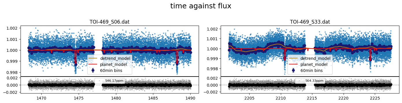
[42]:
fig = result.lc.plot_bestfit(binsize=1/24)
[4]:
result.lc.names
[4]:
['TOI-469_S06.dat', 'TOI-469_S33.dat']
[5]:
#load output data files for the lc fits
lc1data = result.lc.outdata['TOI-469_S06.dat']
lc2data = result.lc.outdata['TOI-469_S33.dat']

lc1data.head()
[5]:
| time | flux | error | full_mod | base_para | base_sine | base_spl | base_gp | base_total | transit | det_flux | residual | phase_1 | phase_2 | phase_3 | |
|---|---|---|---|---|---|---|---|---|---|---|---|---|---|---|---|
| 0 | 1468.276516 | 1.000369 | 0.000546 | 1.000022 | 1.000028 | 0.0 | 1.0 | -0.000007 | 1.000022 | 1.0 | 1.000347 | 0.000347 | -0.461651 | 0.129707 | 0.268246 |
| 1 | 1468.277905 | 1.001143 | 0.000546 | 1.000021 | 1.000028 | 0.0 | 1.0 | -0.000007 | 1.000021 | 1.0 | 1.001122 | 0.001122 | -0.461549 | 0.130099 | 0.268462 |
| 2 | 1468.279293 | 1.000149 | 0.000546 | 1.000021 | 1.000028 | 0.0 | 1.0 | -0.000007 | 1.000021 | 1.0 | 1.000128 | 0.000128 | -0.461447 | 0.130492 | 0.268678 |
| 3 | 1468.280682 | 0.999294 | 0.000545 | 1.000021 | 1.000028 | 0.0 | 1.0 | -0.000007 | 1.000021 | 1.0 | 0.999273 | -0.000727 | -0.461345 | 0.130885 | 0.268894 |
| 4 | 1468.282071 | 0.999478 | 0.000546 | 1.000021 | 1.000028 | 0.0 | 1.0 | -0.000007 | 1.000021 | 1.0 | 0.999457 | -0.000543 | -0.461243 | 0.131277 | 0.269110 |
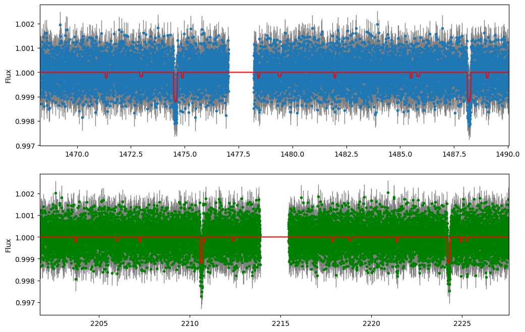
[47]:
fig, ax = plt.subplots(2,1,figsize=(12,8))
ax[0].errorbar(lc1data["time"],lc1data["det_flux"], lc1data["error"],fmt=".", elinewidth=1, ecolor="gray")
ax[0].plot(lc1data.time, lc1data.transit,"r", zorder=5)
ax[0].set_ylabel("Flux");
ax[0].set_xlim([lc1data.time[0], np.array(lc1data.time)[-1]])

ax[1].errorbar(lc2data["time"],lc2data["det_flux"], lc2data["error"],c="g",fmt=".", elinewidth=1, ecolor="gray")
ax[1].plot(lc2data.time, lc2data.transit, "r",zorder=5)
ax[1].set_ylabel("Flux");
ax[1].set_xlim([lc2data.time[0], np.array(lc2data.time)[-1]])
[47]:
(2201.737329, 2227.575994)
[6]:
# join two outputs in a single dataframe (so we can plot the model across the times)
lcdata = pd.concat([lc1data,lc2data])
lcdata.head()
[6]:
| time | flux | error | full_mod | base_para | base_sine | base_spl | base_gp | base_total | transit | det_flux | residual | phase_1 | phase_2 | phase_3 | |
|---|---|---|---|---|---|---|---|---|---|---|---|---|---|---|---|
| 0 | 1468.276516 | 1.000369 | 0.000546 | 1.000022 | 1.000028 | 0.0 | 1.0 | -0.000007 | 1.000022 | 1.0 | 1.000347 | 0.000347 | -0.461651 | 0.129707 | 0.268246 |
| 1 | 1468.277905 | 1.001143 | 0.000546 | 1.000021 | 1.000028 | 0.0 | 1.0 | -0.000007 | 1.000021 | 1.0 | 1.001122 | 0.001122 | -0.461549 | 0.130099 | 0.268462 |
| 2 | 1468.279293 | 1.000149 | 0.000546 | 1.000021 | 1.000028 | 0.0 | 1.0 | -0.000007 | 1.000021 | 1.0 | 1.000128 | 0.000128 | -0.461447 | 0.130492 | 0.268678 |
| 3 | 1468.280682 | 0.999294 | 0.000545 | 1.000021 | 1.000028 | 0.0 | 1.0 | -0.000007 | 1.000021 | 1.0 | 0.999273 | -0.000727 | -0.461345 | 0.130885 | 0.268894 |
| 4 | 1468.282071 | 0.999478 | 0.000546 | 1.000021 | 1.000028 | 0.0 | 1.0 | -0.000007 | 1.000021 | 1.0 | 0.999457 | -0.000543 | -0.461243 | 0.131277 | 0.269110 |
[7]:
# evaluate the transit model across both datasets and get individual planet's transit model
lcmod = result.lc.evaluate(time =np.array(lcdata["time"]), return_std=True,nsamp=1500)
print(vars(lcmod).keys())
dict_keys(['time', 'planet_model', 'components', 'sigma_low', 'sigma_high'])
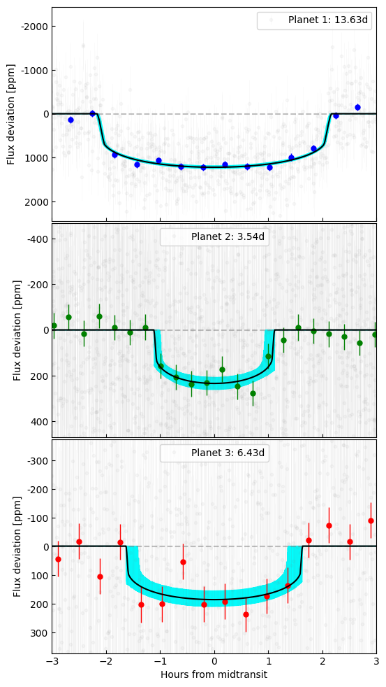
Individual components#
[58]:
lc_comp    = lcmod.components
lc_comp.keys()
[58]:
dict_keys(['pl_1', 'pl_2', 'pl_3'])
[75]:
fig, ax = plt.subplots(3,1, sharex=True, gridspec_kw={'hspace':0.01},figsize=(6,12))

pl = ["pl_1", "pl_2", "pl_3", "pl_1", "pl_2"] #
cl = ["b","g","r"]
n_bin = [800, 300, 400]
for i,n in enumerate(["pl_1", "pl_2", "pl_3"]):
    phase    = phase_fold(  t   = np.array(lcdata["time"]),
                            per = result.params.P[i],
                            t0  = result.params.T0[i],
                            phase0 = -0.5)

    srt = np.argsort(phase)

    pl.remove(n)

    tr_mod          = lc_comp[n]
    subtract_signal = (lc_comp[pl[0]]-1) + (lc_comp[pl[1]]-1) #remove signal from other planets
    planet_signal   = lcdata["det_flux"] - subtract_signal

    p_bin, lc_bin, err_bin = bin_data(phase, planet_signal, lcdata["error"],bins=n_bin[i])

    ax[i].errorbar(   phase*result.params.P[i]*24, planet_signal,  lcdata["error"],
                    fmt=".",c="gray", elinewidth=0.5, alpha=0.05,
                    label=f"Planet {i+1}: {result.params_dict[f'Period_{i+1}'].n:.2f}d")

    ax[i].errorbar(p_bin*result.params.P[i]*24, lc_bin, err_bin, fmt="o",ms=5, c=cl[i], elinewidth=1)

    ax[i].plot(phase[srt]*result.params.P[i]*24, tr_mod[srt],"k",zorder=4)

    lo, hi = np.where(tr_mod==1, 1, lcmod.sigma_low), np.where(tr_mod==1, 1, lcmod.sigma_high)

    ax[i].fill_between( phase[srt]*result.params.P[i]*24,
                        lo[srt],
                        hi[srt],
                        color="cyan"
                        )

    ax[i].legend()
    ax[i].axhline(1,ls="--",c="gray", alpha=0.5)
    ax[i].set_xlabel("Hours from midtransit")
    ax[0].set_ylabel("Flux")
    ax[i].set_xlim([-3,3])
    ax[i].set_ylim([1-2*np.ptp(tr_mod), 1+2*np.ptp(tr_mod)])
    ax[i].tick_params(direction="in")


import matplotlib.ticker as ticker
def ppm_formatter(x, pos):
    """Convert flux to ppm deviation from 1"""
    return f'{(1-x)*1e6:.0f}'

# Apply to existing plot
for i in range(3):
    ax[i].yaxis.set_major_formatter(ticker.FuncFormatter(ppm_formatter))
    ax[i].set_ylabel("Flux deviation [ppm]")
RVS#
[76]:
result.rv.names
[76]:
['TOI469rv1.dat', 'TOI469rv2.dat']
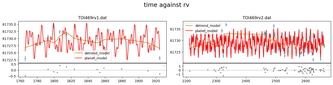
[77]:
fig = result.rv.plot_bestfit()
[78]:
#load output data files for the rv fits
rv1data = result.rv.outdata['TOI469rv1.dat']
rv2data = result.rv.outdata['TOI469rv2.dat']
[79]:
#join two outputs in a single dataframe
rvdata = pd.concat([rv1data,rv2data])
rvdata.head()
[79]:
| time | RV | error | full_mod | base_para | base_spl | base_gp | base_total | Rvmodel | det_RV | gamma | residual | phase_1 | phase_2 | phase_3 | |
|---|---|---|---|---|---|---|---|---|---|---|---|---|---|---|---|
| 0 | 1765.880033 | 81722.91 | 0.807069 | 81723.394084 | 0.0 | 0.0 | -2.225679 | 81726.819770 | -3.425686 | -3.909770 | 81729.045449 | -0.484084 | 0.371466 | 0.246949 | -0.446126 |
| 1 | 1792.789313 | 81730.59 | 0.593431 | 81730.522613 | 0.0 | 0.0 | 0.239247 | 81729.284697 | 1.237916 | 1.305303 | 81729.045449 | 0.067387 | 0.345614 | -0.147178 | -0.260984 |
| 2 | 1799.679952 | 81734.23 | 0.755553 | 81734.363394 | 0.0 | 0.0 | -0.670740 | 81728.374709 | 5.988685 | 5.855291 | 81729.045449 | -0.133394 | -0.148867 | -0.199548 | -0.189298 |
| 3 | 1803.799572 | 81726.85 | 0.588948 | 81727.041896 | 0.0 | 0.0 | 0.436107 | 81729.481556 | -2.439660 | -2.631556 | 81729.045449 | -0.191896 | 0.153361 | -0.035143 | 0.451418 |
| 4 | 1806.664396 | 81732.28 | 0.628379 | 81731.903761 | 0.0 | 0.0 | 1.802835 | 81730.848284 | 1.055478 | 1.431716 | 81729.045449 | 0.376239 | 0.363533 | -0.225404 | -0.103023 |
[80]:
# evaluate the RV model across both datasets
rvmod = result.rv.evaluate(time=np.array(rvdata["time"]), return_std=True, nsamp=1500)
since the RVs are sparsely sampled, we can evaluate the RV model on a smoother time array across both datasets
[81]:
t_sm     = np.linspace(rvdata["time"].min(), rvdata["time"].max(), 2000)
rvmod_sm = result.rv.evaluate(file='TOI469rv1.dat',time=t_sm, return_std=True,nsamp=1500)
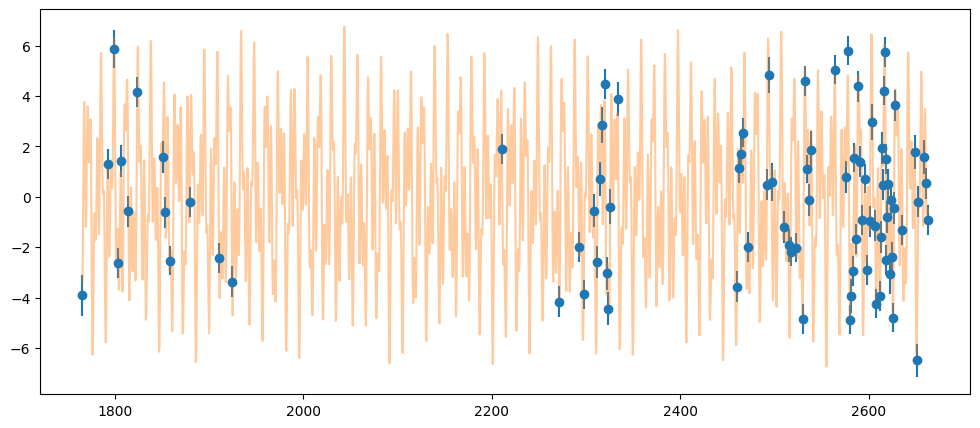
[82]:
plt.figure(figsize=(12,5))
plt.errorbar(rvdata["time"],rvdata["det_RV"], rvdata["error"],fmt="o")
plt.plot(t_sm, rvmod_sm.planet_model, alpha=0.4)
[82]:
[<matplotlib.lines.Line2D at 0x13b7ddde0>]
Individual components#
[85]:
rv_comp    = rvmod.components
rv_comp_sm = rvmod_sm.components
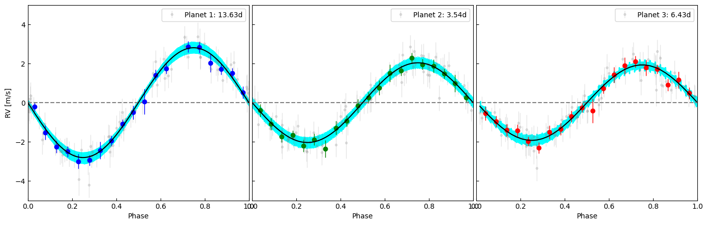
[89]:
fig, ax = plt.subplots(1,3, sharey=True, figsize=(17,5))

pl = ["pl_1", "pl_2", "pl_3", "pl_1", "pl_2"]
cl = ["b","g","r"]
for i,n in enumerate(["pl_1", "pl_2", "pl_3"]):
    phase    = phase_fold(  t   = np.array(rvdata["time"]),
                            per = result.params.P[i],
                            t0  = result.params.T0[i],
                            phase0 = 0)

    phase_sm = phase_fold(  t   = t_sm,
                            per = result.params.P[i],
                            t0  = result.params.T0[i],
                            phase0 = 0)

    srt = np.argsort(phase_sm)

    pl.remove(n)

    subtract_signal    = rv_comp[pl[0]]    + rv_comp[pl[1]]
    subtract_signal_sm = rv_comp_sm[pl[0]] + rv_comp_sm[pl[1]]
    planet_signal      = rvdata["det_RV"]  - subtract_signal

    p_bin, rv_bin, err_bin = bin_data(phase, planet_signal, rvdata["error"],bins=20)

    ax[i].errorbar(   phase, planet_signal,  rvdata["error"],
                    fmt=".",c="gray", elinewidth=1, alpha=0.2,
                    label=f"Planet {i+1}: {result.params_dict[f'Period_{i+1}'].n:.2f}d")

    ax[i].errorbar(p_bin, rv_bin, err_bin, fmt="o", c=cl[i], elinewidth=1)

    ax[i].plot(phase_sm[srt], rv_comp_sm[n][srt],"k",zorder=4)

    ax[i].fill_between( phase_sm[srt],
                        (rvmod_sm.sigma_low - subtract_signal_sm)[srt],
                        (rvmod_sm.sigma_high-subtract_signal_sm)[srt],
                        color="cyan"
                    )

    ax[i].legend()
    ax[i].axhline(0,ls="--",c="gray")
    ax[i].set_xlabel("Phase")
    ax[0].set_ylabel("RV [m/s]")
    ax[i].set_ylim([-5,5])
    ax[i].set_xlim([0,1])
    ax[i].tick_params(direction="in")

plt.subplots_adjust(wspace=0.015)