WASP-127b: Fitting LCs and RVs#
[1]:
from glob import glob
from os.path import basename

import numpy as np
import CONAN
import matplotlib.pyplot as plt
import pandas as pd
CONAN.__version__
[1]:
'3.3.11'
We start by getting the data for the analysis. TESS has observed transits of WASP-127b in many sectors. There are also transits AND RV observations by EULERCAM AND CORALIE on the Swiss telescope.
Download TESS data#
using the lightkurve package, CONAN allows you to query the MAST database and download TESS data
[2]:
from CONAN.get_files import get_TESS_data

df = get_TESS_data("WASP-127")
df.search()
SearchResult containing 25 data products.

 #     mission     year       author      exptime target_name distance
                                             s                 arcsec
--- -------------- ---- ----------------- ------- ----------- --------
  0 TESS Sector 09 2019              SPOC     120   169226822      0.0
  1 TESS Sector 35 2021              SPOC      20   169226822      0.0
  2 TESS Sector 46 2021              SPOC     120   169226822      0.0
  3 TESS Sector 35 2021              SPOC     120   169226822      0.0
  4 TESS Sector 72 2023              SPOC      20   169226822      0.0
  5 TESS Sector 62 2023              SPOC      20   169226822      0.0
  6 TESS Sector 72 2023              SPOC     120   169226822      0.0
  7 TESS Sector 62 2023              SPOC     120   169226822      0.0
  8 TESS Sector 89 2025              SPOC      20   169226822      0.0
...            ...  ...               ...     ...         ...      ...
 15 TESS Sector 09 2019               QLP    1800   169226822      0.0
 16 TESS Sector 46 2021               QLP     600   169226822      0.0
 17 TESS Sector 35 2021               QLP     600   169226822      0.0
 18 TESS Sector 72 2023               QLP     200   169226822      0.0
 19 TESS Sector 62 2023               QLP     200   169226822      0.0
 20 TESS Sector 89 2025               QLP     200   169226822      0.0
 21 TESS Sector 09 2019              TGLC    1800   169226822      0.0
 22 TESS Sector 09 2019 GSFC-ELEANOR-LITE    1800   169226822      0.0
 23 TESS Sector 46 2021             CDIPS    1800   169226822      0.0
 24 TESS Sector 35 2021             CDIPS    1800   169226822      0.0
Length = 25 rows
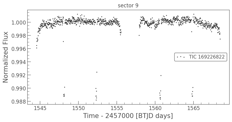
Let’s go with long cadence (600s) data so we can try supersampling with CONAN
[3]:
df.download(sectors=[9],author="TESS-SPOC", exptime=1800,
            select_flux="pdcsap_flux",quality_bitmask='hardest')
downloaded lightcurve for sector 9
[4]:
df.scatter()
[6]:
df.save_CONAN_lcfile(bjd_ref = 2450000, folder="../data")
saved file as: ../data/WASP-127_S9.dat
CONAN Brief#
The CONAN has 3 major classes that are used to store information about the input files and setup fit configuration.
They are:
load_lightcurves(): ingest lightcurve files and creates an object that is used to configure baseline and model parameters. It contains methods to configure the LCs for fitting such as:lc_baseline()get_decorr()add_GP()add_spline()add_sinusoid()supersample()clip_outliers()add_custom_LC_function()planet_parameters()phasecurve()transit_depth_variation()transit_timing_variation()limb_darkening()get_LDs()Save_LCs()…
load_rvs: similar to above that are applicable to RVsfit_setup: object to setup sampling of the parameter space
These objects are then given as input to the run_fit() function to perform sampling and the outcome saved as a result object.
Setup light curve object#
We will fit one Euler lightcurve and the tess sector 9 lightcurve
[2]:
path = "../data/"     #path to the lightcurve files
lc_list  = ["lc6bjd.dat", "WASP-127_S9.dat"]
load light curve into CONAN and visualize#
[3]:
lc_obj = CONAN.load_lightcurves( file_list     = lc_list,
                                  data_filepath = path,
                                  filters       = ["R","T"],
                                  wl            = [0.6, 0.8], #in microns, only used to plot depth differences
                                  nplanet       = 1)
lc_obj
# ============ Input lightcurves, filters baseline function =======================================================
name            flt 𝜆_𝜇m |Ssmp ClipOutliers scl_col |off col0 col3 col4 col5 col6 col7 col8|sin id GP spline
lc6bjd.dat      R   0.6  |None None         None    |  y    0    0    0    0    0    0    0|n    1 n  None
WASP-127_S9.dat T   0.8  |None None         None    |  y    0    0    0    0    0    0    0|n    2 n  None
[3]:
lightcurves from filepath: ../data/
1 transiting planet(s)
Order of unique filters: ['R', 'T']
The lightcurve object
lc_objholds information about the light curves (data and settings):
Ssmp: supersampling (for long cadence data)
clip: outlier clipping
scl_col: scaling the arrays in the columns of the data
off: whether to fit for an offset
col{x}: polynomial order in the columns x={0,3,4,5,6,7} of the data to use for decorrelation
sin: include a sinusoid in the baseline model
id: light curve number
GP: defined GP to model the baseline
spline_config: fit a spline to the baseline
By default they are all deactivated. We will define these different options in the following steps
We can inspect the light curve files which are stored as dictionary in lc_obj._input_lc.
Use pandas just for nice print-out of the first 5 lines and see the assigned column names
[4]:
pd.DataFrame(lc_obj._input_lc["lc6bjd.dat"]).head()
[4]:
| col0 | col1 | col2 | col3 | col4 | col5 | col6 | col7 | col8 | |
|---|---|---|---|---|---|---|---|---|---|
| 0 | 8209.555598 | 1.007264 | 0.000705 | 2.43 | 4.48 | 1.20 | 15.11 | 284.40 | 45.0 |
| 1 | 8209.556263 | 1.006767 | 0.000704 | 0.52 | 2.49 | 1.20 | 15.71 | 284.47 | 45.0 |
| 2 | 8209.556931 | 1.007128 | 0.000704 | 0.46 | 2.78 | 1.20 | 15.02 | 284.95 | 45.0 |
| 3 | 8209.557602 | 1.007728 | 0.000705 | 1.63 | 1.94 | 1.20 | 15.46 | 283.68 | 45.0 |
| 4 | 8209.558277 | 1.005616 | 0.000697 | 1.94 | 1.78 | 1.19 | 15.98 | 285.25 | 45.0 |
[5]:
pd.DataFrame(lc_obj._input_lc["WASP-127_S9.dat"]).head()
[5]:
| col0 | col1 | col2 | col3 | col4 | col5 | col6 | col7 | col8 | |
|---|---|---|---|---|---|---|---|---|---|
| 0 | 8544.537364 | 0.996105 | 0.000231 | 1.0 | 1.0 | 1.0 | 1.0 | 1.0 | 1.0 |
| 1 | 8544.558198 | 0.996479 | 0.000230 | 1.0 | 1.0 | 1.0 | 1.0 | 1.0 | 1.0 |
| 2 | 8544.579031 | 0.997080 | 0.000230 | 1.0 | 1.0 | 1.0 | 1.0 | 1.0 | 1.0 |
| 3 | 8544.599865 | 0.997540 | 0.000230 | 1.0 | 1.0 | 1.0 | 1.0 | 1.0 | 1.0 |
| 4 | 8544.620698 | 0.997604 | 0.000229 | 1.0 | 1.0 | 1.0 | 1.0 | 1.0 | 1.0 |
Notice that col3 to col8 of the TESS data were automatically filled with ones since they were empty
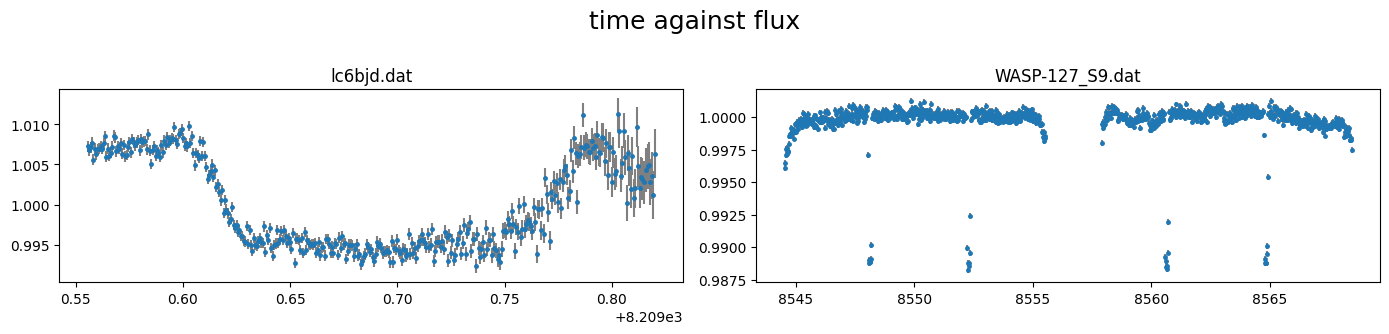
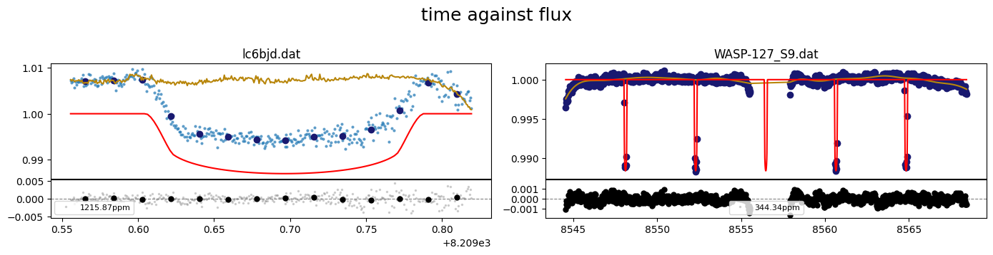
The light curves can be plotted using the plot() method of the object.
By default this plots column 0 (time) against column 1 (flux) with column 3(flux err) as uncertainties.
[6]:
lc_obj.plot()
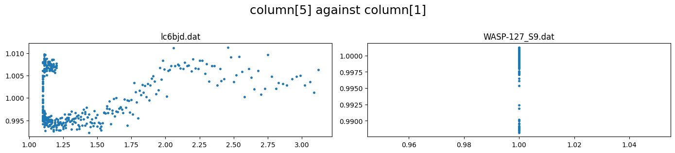
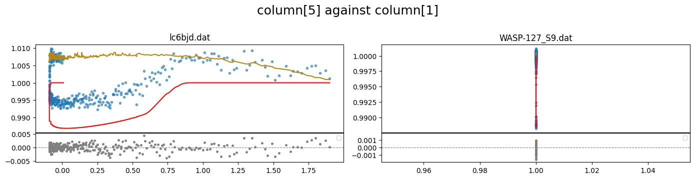
correlations between the flux and other columns in the lightcurve file can be visualized by specifying the columns to plot. e.g. to plot column5 against column 1 (flux)
[7]:
lc_obj.plot(plot_cols=(5,1))
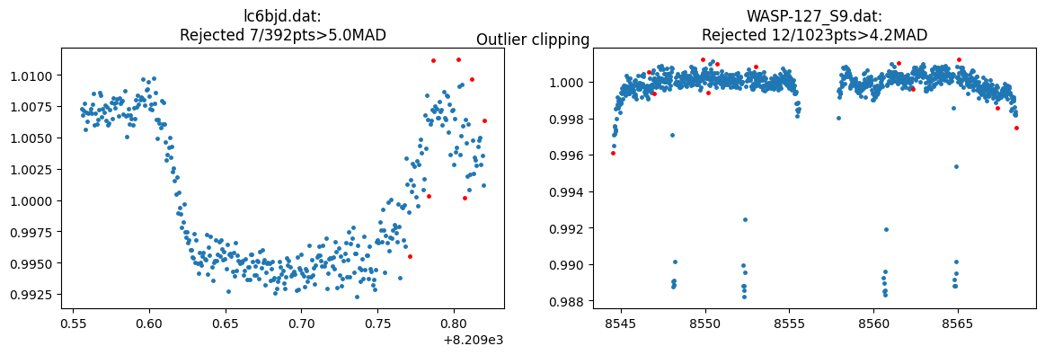
some data processing#
we can remove outliers from all or specific lcs. This uses a sliding median of specified width to discard points greater than clip\(\times\) the M.A.D (median absoulte deviation). The clipped data is saved to the lc_obj. further analysis is performed on the clipped data
[8]:
lc_obj.clip_outliers(lc_list="all", width=[11,5], clip=[5,4.2],show_plot=True)
This is useful for decorrelating the flux against the different columns. It is only performed on columns 3 and above whose values do not span zero. There are 3 methods to rescale the data: “med_sub”, “rs0to1”, “rs-1to1” which subtracts the median, rescales to [0-1], or rescales to [-1,1] respectively
[9]:
lc_obj.rescale_data_columns(method=["med_sub","None"])
Rescaled data columns of lc6bjd.dat with method:med_sub
No rescaling for WASP-127_S9.dat
We can confirm that these operations have been written into lc_obj
[10]:
lc_obj
# ============ Input lightcurves, filters baseline function =======================================================
name            flt 𝜆_𝜇m |Ssmp ClipOutliers scl_col |off col0 col3 col4 col5 col6 col7 col8|sin id GP spline
lc6bjd.dat      R   0.6  |None c1:W11C5n1   med_sub |  y    0    0    0    0    0    0    0|n    1 n  None
WASP-127_S9.dat T   0.8  |None c1:W5C4.2n1  None    |  y    0    0    0    0    0    0    0|n    2 n  None
[10]:
lightcurves from filepath: ../data/
1 transiting planet(s)
Order of unique filters: ['R', 'T']
showing the med_sub has been used to scale the relevant columns of lc6bjd.dat, and the data have been clipped using c{``column``}:W{``width``}C{``clip``}n{``iterations``}
For each loaded light curve, the rms and jitter are estimated from the data properties and stored in a list as:
[11]:
print(f"{lc_obj._rms_estimate  = }")
print(f"{lc_obj._jitt_estimate = }")
lc_obj._rms_estimate  = [0.0011117820828712038, 0.00028087567717406876]
lc_obj._jitt_estimate = [0.0003490563305132201, 0.00017317313538562336]
the jitter estimates the amount of extra noise to be quadratically added to the flux errorbars for them to be commensurate to the flux rms. For each lc, the log of this value is used as start value when fitting the log_jitter. The user can modify this list as required
the rms_estimate is used to define limits on the decorrelation parameters if not defined by user
Setup Transit#
Parameters are defined in CONAN in 4 formats:
Fixed: int/float e.g
q1= 0.5Normal prior: tuple of length 2 –> (mean, sigma) e.g.
rho_star= (0.5, 0.03)Uniform prior: tuple of length 3 –> (min, start, max) e.g.
Period= (0, 0.5, 1)LogUniform prior: tuple of length 4 –> (min, start, max,’LU’) e.g.
rho_star= (0.01, 1, 100, ‘LU’)truncated normal prior: tuple of length 4 –> (min, max, mu, sigma) e.g
q1=(0,1,0.2,0.1)
We can get system parameters from the NASA exoplanet archive
[12]:
from CONAN.get_files import get_parameters

sys_params = get_parameters(planet_name   ="WASP-127b",
                            check_rhostar =True)  #result cached in the current working directory
sys_params
Getting system parameters from NASA exoplanet archive ...
rho_star to Tdur: 0.175718+/-0.002816
T14:              0.181370+/-0.000350
rho_star conversion to Tdur is consistent with literature T14 within 3 sigma
[12]:
{'star': {'Teff': (5620.0, 85.0),
  'logg': (4.18, 0.01),
  'FeH': (-0.193, 0.014),
  'radius': (1.333, 0.027),
  'mass': (0.95, 0.02),
  'density': (0.569, 0.021)},
 'planet': {'name': 'WASP-127 b',
  'period': (4.17806203, 8.8e-07),
  'rprs': (0.10103, 0.00026),
  'mass': (0.1647, 0.0214),
  'ecc': (0.0, nan),
  'w': (nan, nan),
  'T0': (2456776.62124, 0.00023),
  'b': (0.29, 0.04),
  'T14': (0.18137, 0.00035),
  'aR': (7.81, 0.11),
  'K[m/s]': (22.0, 3.0)}}
The sys_params can be used to specify the priors for the planet’s transit and RV parameters
Let’s put the relevant planet parameters in a dictionary for convenience. The parameters are defined for transit/occultation/phasecurve/rv
[13]:
t0  = sys_params["planet"]["T0"][0] - 2450000

planet_pars = dict( T_0           = (t0, 0.001),                           #normal prior
                    Period        = sys_params["planet"]["period"][0],     #fixed
                    rho_star      = sys_params["star"]["density"],         #normal pripr
                    Impact_para   = (0, sys_params["planet"]["b"][0], 1),  #uniform prior
                    RpRs          = (0.05, 0.108, 0.17),                   #uniform prior
                    Eccentricity  = 0,
                    omega         = 90,
                    K             = 0)
The .planet_parameters() method of lc_obj is called to define the parameters in CONAN. This method takes in the same parameter names as defined in planet_pars dictionary so we can load this directly
[14]:
lc_obj.planet_parameters(**planet_pars)
# ============ Planet parameters (Transit and RV) setup ==========================================================
name                       fit  prior                                   note
[rho_star]/Duration        y    N(0.569,0.021)                          #choice in []|unit(gcm^-3/days)
--------repeat this line & params below for multisystem, adding '_planet_number' to the names e.g RpRs_1 for planet 1, ...
RpRs                       y    U(0.05,0.108,0.17)                      #range[-0.5,0.5]
Impact_para                y    U(0,0.29,1)                             #range[0,2]
T_0                        y    N(6776.621239999775,0.001)              #unit(days)
Period                     n    F(4.17806203)                           #range[0,inf]days
[Eccentricity]/sesinw      n    F(0)                                    #choice in []|range[0,1]/range[-1,1]
[omega]/secosw             n    F(90)                                   #choice in []|range[0,360]deg/range[-1,1]
K                          n    F(0)                                    #unit(same as RVdata)
rho_star or Duration can be supplied. the user selection is given in square brackets.
The same goes for Eccentricity–omega combination which can instead be sesinw–secosw
The
sys_paramscan also be used to obtain priors on the stellar limb darkening from the phoenix stellar library.CONANuses the Kipping parameterization of the quadratic law defined as \(q_1\) and \(q_2\).
Filter names can be obtained from the SVO filter service with names such as Spitzer/IRAC.I1 or a name shortcut such as TESS, CHEOPS,kepler.
List of filter shortcut names can be obtained using:
[15]:
lc_obj._filter_shortcuts
[15]:
{'kepler': 'Kepler/Kepler.k',
 'tess': 'TESS/TESS.Red',
 'cheops': 'CHEOPS/CHEOPS.band',
 'wfc3_g141': 'HST/WFC3_IR.G141',
 'wfc3_g102': 'HST/WFC3_IR.G102',
 'sp36': 'Spitzer/IRAC.I1',
 'sp45': 'Spitzer/IRAC.I2',
 'ug': 'Geneva/Geneva.U',
 'b1': 'Geneva/Geneva.B1',
 'b2': 'Geneva/Geneva.B2',
 'bg': 'Geneva/Geneva.B',
 'gg': 'Geneva/Geneva.G',
 'v1': 'Geneva/Geneva.V2',
 'vg': 'Geneva/Geneva.V',
 'sdss_g': 'SLOAN/SDSS.g',
 'sdss_r': 'SLOAN/SDSS.r',
 'sdss_i': 'SLOAN/SDSS.i',
 'sdss_z': 'SLOAN/SDSS.z'}
we specify filters for the EULER and TESS data
[16]:
# the filter names assigned to each data during lightcurve ingestion are:
lc_obj._filnames
[16]:
array(['R', 'T'], dtype='<U1')
[17]:
filts = ['sdss_r','tess']
[18]:
print(f"\nGetting limb darkening parameters for filter {filts}")
q1, q2 = lc_obj.get_LDs( Teff = sys_params['star']['Teff'],
                        logg  = sys_params['star']['logg'],
                        Z     = sys_params['star']['FeH'],
                        filter_names=filts)
Getting limb darkening parameters for filter ['sdss_r', 'tess']
sdss_r    (R): q1=(0.4221, 0.0227), q2=(0.3963, 0.0145)
tess      (T): q1=(0.2973, 0.0148), q2=(0.3782, 0.0131)
[19]:
print(f"{q1=}\n{q2=}")
q1=[(0.4221, 0.0227), (0.2973, 0.0148)]
q2=[(0.3963, 0.0145), (0.3782, 0.0131)]
q1, q2 can then be passed to the .limb_darkening() method of lc_obj
[20]:
lc_obj.limb_darkening(q1=q1, q2=q2)
# ============ Limb darkening setup =============================================================================
filters fit     q1                      q2
R       y       N(0.4221,0.0227)        N(0.3963,0.0145)
T       y       N(0.2973,0.0148)        N(0.3782,0.0131)
Baseline and decorrelation parameters#
The baseline model for each lightcurve in lc_obj object can be defined manually or automagically
We manually define the baseline model using the .lc_baseline() method of the lc_obj
Define baseline model parameters to fit for each light curve using the columns of the input data. dcol0 refers to decorrelation setup for column 0, dcol3 for column 3, and so on.
Each baseline decorrelation parameter (dcol{x}) should be a list of integers specifying the polynomial order for column {x} for each light curve. e.g. Given 2 input light curves as we have here,
If one wishes to fit a 1st order trend in column 0 (time) to only the first and second lightcurve, then dcol0 = [1, 1].
For the first lightcurve, we saw a strong correlation of the flux with column 5. We can fit this with a 2nd order term by setting dcol5 = [2, 0]
[21]:
lc_obj.lc_baseline( dcol0 = [1, 1],
                    dcol5 = [2, 0],
                    )
# ============ Input lightcurves, filters baseline function =======================================================
name            flt 𝜆_𝜇m |Ssmp ClipOutliers scl_col |off col0 col3 col4 col5 col6 col7 col8|sin id GP spline
lc6bjd.dat      R   0.6  |None c1:W11C5n1   med_sub |  y    1    0    0    2    0    0    0|n    1 n  None
WASP-127_S9.dat T   0.8  |None c1:W5C4.2n1  None    |  y    1    0    0    0    0    0    0|n    2 n  None
we can add a spline to the baseline of the TESS lc using the
.add_spline()method
Let’s add a spline of degree 3 in time (col0) to the baseline model of the TESS data. A spline is fitted to consecutive knot_spacing chunks of the data.
[22]:
lc_obj.add_spline(  lc_list      = ["WASP-127_S9.dat"],
                    par          = ["col0"],
                    degree       = [3],
                    knot_spacing = [2])
# ============ Input lightcurves, filters baseline function =======================================================
name            flt 𝜆_𝜇m |Ssmp ClipOutliers scl_col |off col0 col3 col4 col5 col6 col7 col8|sin id GP spline
lc6bjd.dat      R   0.6  |None c1:W11C5n1   med_sub |  y    1    0    0    2    0    0    0|n    1 n  None
WASP-127_S9.dat T   0.8  |None c1:W5C4.2n1  None    |  n    1    0    0    0    0    0    0|n    2 n  c0:d3k2
Notice that the addition of a spline to the TESS data sets off="n" for that lc. that’s because the spline model already contains an offset term thereby making the off here unnecessary
Let’s also supersample the long cadence TESS data by a factor of 30 (
x30.0). This subdivides each exposure time by 30 to attain a sampling of ~1 minute. We can use a supersampling facore ofx15to acheive 2 minute sampling.
[23]:
lc_obj.supersample( lc_list   = ["WASP-127_S9.dat"],
                    ss_factor = 30)
Supersampling WASP-127_S9.dat with exp_time=30.0mins each divided into 30 subexposures
# ============ Input lightcurves, filters baseline function =======================================================
name            flt 𝜆_𝜇m |Ssmp ClipOutliers scl_col |off col0 col3 col4 col5 col6 col7 col8|sin id GP spline
lc6bjd.dat      R   0.6  |None c1:W11C5n1   med_sub |  y    1    0    0    2    0    0    0|n    1 n  None
WASP-127_S9.dat T   0.8  |x30  c1:W5C4.2n1  None    |  n    1    0    0    0    0    0    0|n    2 n  c0:d3k2
Figuring out the best combination of decorrelation parameters for each lightcurve can be quite difficult requiring to perform several fits to the data and somehow select the fit with the best decorrelation. CONAN implements a method to determine the best baseline model for each input lightcurve
The .get_decorr() function of the lc_obj can be used to automatically determine the best decorrelation parameters to use. This is a least-squares fit (using lmfit package) to the data and comparing the Bayesian Information Criterion, BIC, when adding decorrelation parameters (see forward selection regression method )
To do this, we would like take into account the transit/occultation/phasecurve when peforming the least-squares fit. So defined parameter priors in planet_pars are also used
Now run .get_decorr() to get decorrelation parameters by loading the planet_pars dictionary and limb darkening priors q1,q2.
The function uses columns 0,3,4,5,6,7 to construct a polynomial trend model. The decorr parameters are labelled Ai,Bi for 1st & 2nd order coefficients in column i.
spline,supersampling, and GP configurations are also used for decorrelation, if defined before running .get_decorr()
By default, decorrelation parameters that reduce the BIC by 5 (i.e delta_BIC = -5) are iteratively selected. This implies bayes_factor = \(e^{(-0.5 \times -5)}\) = 12 or more is required for a parameter to be selected.
[24]:
decorr_res = lc_obj.get_decorr( **planet_pars,
                                q1             = q1,
                                q2             = q2,
                                exclude_cols   = [7],       #columns to exclude from decorrelation e.g [3,4]
                                enforce_pars   = [],       #decorr parameters to enforce e.g ["A5",B6]
                                delta_BIC      = -5,
                                setup_baseline = True,
                                show_steps     = False,
                                )
getting decorr params for lc01: lc6bjd.dat (spline=False, sine=False, gp=False, s_samp=False, jitt=0.0ppm)
BEST BIC:710.68, pars:['offset', 'A6', 'B5', 'A5']

getting decorr params for lc02: WASP-127_S9.dat (spline=True, sine=False, gp=False, s_samp=True, jitt=0.0ppm)
BEST BIC:2495.81, pars:['B0', 'A0']

Setting-up parametric baseline model from decorr result
# ============ Input lightcurves, filters baseline function =======================================================
name            flt 𝜆_𝜇m |Ssmp ClipOutliers scl_col |off col0 col3 col4 col5 col6 col7 col8|sin id GP spline
lc6bjd.dat      R   0.6  |None c1:W11C5n1   med_sub |  y    0    0    0    2    1    0    0|n    1 n  None
WASP-127_S9.dat T   0.8  |x30  c1:W5C4.2n1  None    |  n    2    0    0    0    0    0    0|n    2 n  c0:d3k2
Total number of baseline parameters: 6
the output decorr_res is a list that holds the lmfit result for each lc. Explore each element to see the result
[25]:
decorr_res
[25]:
[<lmfit.minimizer.MinimizerResult at 0x1404639d0>,
 <lmfit.minimizer.MinimizerResult at 0x13ff0bd30>]
We can use the .plot() method again to visualize the fit quality across the different decorrelation axis by setting show_decorr_model=True
[26]:
lc_obj.plot(plot_cols=(5,1), show_decorr_model=True)
[27]:
lc_obj.plot(plot_cols=(0,"res"), show_decorr_model=True)
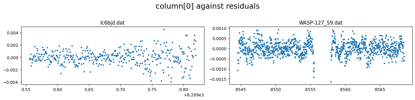
We see that the residuals from the TESS lightcurve fit still has correlated structures that the spline fit did not do very well in capturing
We can remove the spline fitting for TESS and instead use a Celerite GP for the baseline
[28]:
lc_obj.add_spline(None)
No spline
We can use the .print() method to print out the current configuration of the different sections of the lc_obj
To see the current baseline model configuration, set section to “lc_baseline”
[29]:
lc_obj.print(section="lc_baseline")
# ============ Input lightcurves, filters baseline function =======================================================
name            flt 𝜆_𝜇m |Ssmp ClipOutliers scl_col |off col0 col3 col4 col5 col6 col7 col8|sin id GP spline
lc6bjd.dat      R   0.6  |None c1:W11C5n1   med_sub |  y    0    0    0    2    1    0    0|n    1 n  None
WASP-127_S9.dat T   0.8  |x30  c1:W5C4.2n1  None    |  n    2    0    0    0    0    0    0|n    2 n  None
Notice that the spline_config has been set to None for the TESS data
Define GP#
The .add_GP() method of lc_obj is used to setup GP for the lightcurves - selecting the GP package to use, the kernels and priors on the hyperparameters.
GP package gp_pck can be one of [“ge”,”ce”,”sp”] for George, Celerite, or Spleaf.
GP kernel options are:
George: [‘mat32’, ‘mat52’, ‘exp’, ‘cos’, ‘expsq’, ‘exps2’, ‘qp’, ‘rquad’]
Celerite: [‘mat32’, ‘exp’, ‘cos’, ‘sho’, ‘qp_ce’]
Spleaf: [‘mat32’, ‘mat52’, ‘exp’, ‘cos’, ‘sho’, ‘expsq’, ‘exps2’, ‘qp’, ‘qp_sc’, ‘qp_mp’]
see details of the kernel definitions on the github wiki
Up to 2 kernels of the same package can be used for each lc and then their sum or product can be taken.
2 GP hyperparameters are to be specified: amplitude corresponds to the standard deviation of the noise process in ppm, and lengthscale corresponds to the characteristic timescale of the noise process.
[30]:
lc_obj.add_GP(lc_list     = ["WASP-127_S9.dat"],
              par         = ["col0"],
              kernel      = ["mat32"],
              amplitude   = [(20,400, 4000)],    #in ppm, uses log-uniform prior
              lengthscale = [(0.007,0.4, 5)],    #in days, also log-uniform prior
              gp_pck      = ["ce"]               ## gp package celerite
              )
# ============ Input lightcurves, filters baseline function =======================================================
name            flt 𝜆_𝜇m |Ssmp ClipOutliers scl_col |off col0 col3 col4 col5 col6 col7 col8|sin id GP spline
lc6bjd.dat      R   0.6  |None c1:W11C5n1   med_sub |  y    0    0    0    2    1    0    0|n    1 n  None
WASP-127_S9.dat T   0.8  |x30  c1:W5C4.2n1  None    |  n    2    0    0    0    0    0    0|n    2 ce None
# ============ Photometry GP properties (start newline with name of * or + to Xply or add a 2nd gp to last file) =========
name/filt       kern  par    h1:[Amp_ppm]       h2:[len_scale1]    h3:[Q,η,α,b]       h4:[P]
WASP-127_S9.dat mat32 col0   LU(20,400,4000)    LU(0.007,0.4,5)    None               None
[31]:
lc_obj.transit_depth_variation()
lc_obj.phasecurve()
lc_obj.contamination_factors()
# ============ ddF setup ========================================================================================
Fit_ddFs        dRpRs                   div_white
n               U(-0.5,0,0.5)           n
R: modeling only occultation signal
T: modeling only occultation signal
# ============ Phase curve setup ================================================================================
flt D_occ[ppm]         Fn[ppm]            ph_off[deg]  A_ev[ppm]       f1_ev[ppm]    A_db[ppm]       pc_model
R   F(0)               None               None         F(0)            F(0)          F(0)            cosine
T   F(0)               None               None         F(0)            F(0)          F(0)            cosine
# ============ contamination setup (give contamination as flux ratio) ========================================
flt     contam_factor
R       F(0)
T       F(0)
visualize all light curve setup or different sections#
[32]:
lc_obj.print("limb_darkening")
# ============ Limb darkening setup =============================================================================
filters fit     q1                      q2
R       y       N(0.4221,0.0227)        N(0.3963,0.0145)
T       y       N(0.2973,0.0148)        N(0.3782,0.0131)
[ ]:
 #no argument prints all lightcurve setup
lc_obj.print()
Setup RV#
The RV setup is similar to the LC
[34]:
path ="../data/"
rv_list = ["rv1.dat","rv2.dat"]    #rv data in km/s
[35]:
rv_obj = CONAN.load_rvs(file_list     = rv_list,
                         data_filepath = path,
                         rv_unit       ='km/s',
                         nplanet       = 1,
                         lc_obj        = lc_obj      #load lc_obj if planning to update planet parameters
                        )
rv_obj
# ============ Input RV curves, baseline function, GP, spline,  gamma ============================================
name    RVunit scl_col |col0 col3 col4 col5| sin GP spline_config   | gamma_km/s
rv1.dat km/s   None    |   0    0    0    0|   0 n  None            | F(0.0)
rv2.dat km/s   None    |   0    0    0    0|   0 n  None            | F(0.0)
[35]:
rvs from filepath: ../data/
1 planet(s)
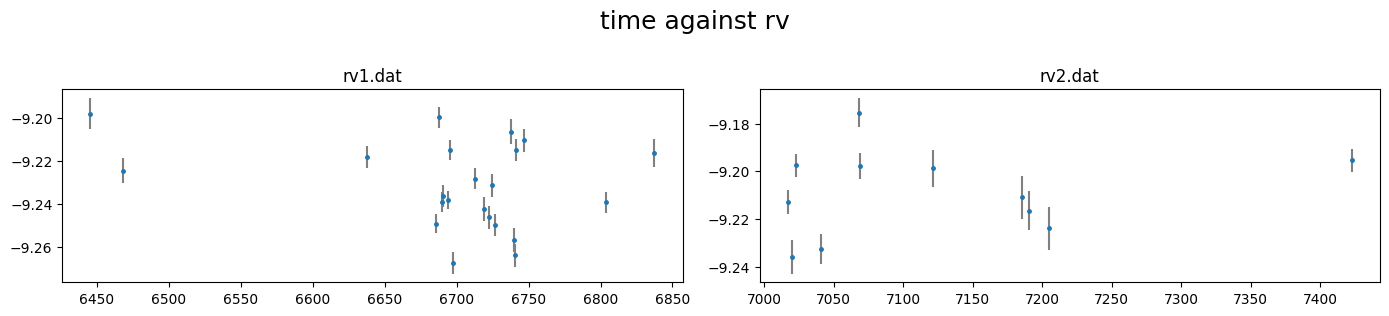
[36]:
rv_obj.plot()
[37]:
pd.DataFrame(rv_obj._input_rv["rv1.dat"]).head()
[37]:
| col0 | col1 | col2 | col3 | col4 | col5 | |
|---|---|---|---|---|---|---|
| 0 | 6445.543512 | -9.197929 | 0.007287 | -0.042628 | 8.150114 | 34.211741 |
| 1 | 6468.462797 | -9.224495 | 0.005818 | -0.036697 | 8.192204 | 33.604743 |
| 2 | 6637.825616 | -9.218248 | 0.005210 | -0.035312 | 8.191037 | 33.948751 |
| 3 | 6685.729323 | -9.249265 | 0.004468 | -0.034618 | 8.264129 | 33.534162 |
| 4 | 6687.689793 | -9.199722 | 0.005097 | 0.000972 | 8.288035 | 33.353229 |
[38]:
rv_obj.rescale_data_columns()
Rescaled data columns of rv1.dat with method:med_sub
Rescaled data columns of rv2.dat with method:med_sub
We can update the RV parameters incase not defined in lc_obj.planet_parameters()
e.g. add a prior for the RV semi-amplitude K
[39]:
rv_obj.update_planet_parameters(K=(0,10e-3,50e-3))
# ============ Planet parameters (Transit and RV) setup ==========================================================
name                       fit  prior                                   note
[rho_star]/Duration        y    N(0.569,0.021)                          #choice in []|unit(gcm^-3/days)
--------repeat this line & params below for multisystem, adding '_planet_number' to the names e.g RpRs_1 for planet 1, ...
RpRs                       y    U(0.05,0.108,0.17)                      #range[-0.5,0.5]
Impact_para                y    U(0,0.29,1)                             #range[0,2]
T_0                        y    N(6776.621239999775,0.001)              #unit(days)
Period                     n    F(4.17806203)                           #range[0,inf]days
[Eccentricity]/sesinw      n    F(0)                                    #choice in []|range[0,1]/range[-1,1]
[omega]/secosw             n    F(90)                                   #choice in []|range[0,360]deg/range[-1,1]
K                          y    U(0,0.01,0.05)                          #unit(same as RVdata)
Baseline and decorrelation#
similar to lightcurves, we can manually specify the rv baseline model using the
.rv_baseline()method
[40]:
rv_obj.rv_baseline( dcol0 = None,
                    dcol3 = None,
                    dcol4 = None,
                    dcol5 = None,
                    gamma = [(-9.232,0.1), (-9.21,0.1)],
                    gp    = "n")
# ============ Input RV curves, baseline function, GP, spline,  gamma ============================================
name    RVunit scl_col |col0 col3 col4 col5| sin GP spline_config   | gamma_km/s
rv1.dat km/s   med_sub |   0    0    0    0|   0 n  None            | N(-9.232,0.1)
rv2.dat km/s   med_sub |   0    0    0    0|   0 n  None            | N(-9.21,0.1)
or we can use the
.get_decorr()method to find the best decorrelation
[41]:
rvdecorr_res= rv_obj.get_decorr(T_0     = planet_pars["T_0"][0],
                                Period  = planet_pars["Period"],
                                K       = (0,22e-3,100e-3),       #km/s
                                gamma   = (-9.21,0.1),            #km/s
                                delta_BIC = -3)
getting decorr params for rv01: rv1.dat (jitt=0.00km/s)

BEST BIC:76.55, pars:['B0', 'A3', 'A4']

getting decorr params for rv02: rv2.dat (jitt=0.00km/s)

BEST BIC:14.02, pars:[]
Setting-up rv baseline model from result
# ============ Input RV curves, baseline function, GP, spline,  gamma ============================================
name    RVunit scl_col |col0 col3 col4 col5| sin GP spline_config   | gamma_km/s
rv1.dat km/s   med_sub |   2    1    1    0|   0 n  None            | N(-9.229240663522978,0.1)
rv2.dat km/s   med_sub |   0    0    0    0|   0 n  None            | N(-9.210554832957529,0.1)
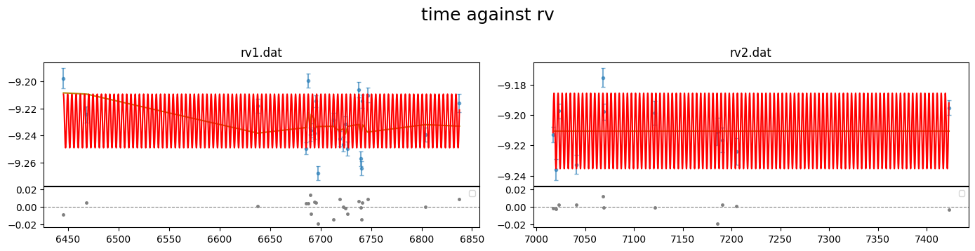
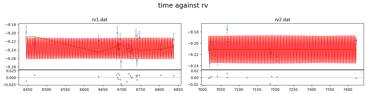
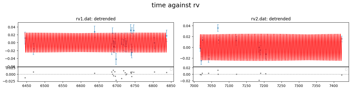
[42]:
rv_obj.plot(plot_cols         = (0,1,2),
            show_decorr_model = True,
            detrend           = True,
            phase_plot        = 1 )
investigate the reduced chi-square of the fits
[43]:
rvdecorr_res[0].redchi, rvdecorr_res[1].redchi
[43]:
(3.593688666537606, 1.0248418035114055)
the high redchi of the first RV data implies that it needs a more complicated baseline model or the errorbars are underestimated. we will fit for an RV jitter for each data in the global fit.
if there are no RV for the setup, it can be turned off using:
[44]:
# rv_data = CONAN.load_rvs()
Setup Sampling#
finally to setup the fit_obj which is used to configure the fitting.
We can specify values for the stellar mass or radius to be used to convert parameter results to physical values. These values are not used in the fit, only for the post-fit conversion. We can also take the values from our NASA archive sys_params dictionary
[45]:
sys_params["star"]["radius"], sys_params["star"]["mass"]
[45]:
((1.333, 0.027), (0.95, 0.02))
[46]:
fit_obj = CONAN.fit_setup(  R_st            = sys_params["star"]["radius"],
                            M_st            = sys_params["star"]["mass"],
                            par_input       = "Rrho",
                            apply_LCjitter  = "y",
                            apply_RVjitter  = "y",
                            LCbasecoeff_lims= "auto",
                            RVbasecoeff_lims= "auto")
# ============ Stellar input properties ======================================================================
# parameter     value
Radius_[Rsun]  N(1.333,0.027)
Mass_[Msun]    N(0.95,0.02)
Input_method:[R+rho(Rrho), M+rho(Mrho)]: Rrho
setup sampling using the .sampling() method of fit_obj. Note that the sampling of the parameter space can be done with emcee or dynesty. The default is dynesty
[47]:
fit_obj.sampling(sampler="dynesty",n_cpus=10, n_live=100)
# ============ FIT setup =====================================================================================
Number_steps                              2000
Number_chains                             64
Number_of_processes                       10
Burnin_length                             500
n_live                                    100
force_nlive                               False
d_logz                                    0.1
Sampler(emcee/dynesty)                    dynesty
emcee_move(stretch/demc/snooker)          stretch
nested_sampling(static/dynamic[pfrac])    static
leastsq_for_basepar(y/n)                  n
apply_LCjitter(y/n,list)                  y
apply_RVjitter(y/n,list)                  y
LCjitter_loglims(auto/[lo,hi])            auto
RVjitter_lims(auto/[lo,hi])               auto
LCbasecoeff_lims(auto/[lo,hi])            auto
RVbasecoeff_lims(auto/[lo,hi])            auto
Light_Travel_Time_correction(y/n)         n
Export configuration#
All configuration can be exported to a config.dat file that allows to reproduce all steps and eventually run the fit
[57]:
CONAN.create_configfile(   lc_obj   = lc_obj,
                            rv_obj   = rv_obj,
                            fit_obj  = fit_obj,
                            filename = 'wasp127_lcrv_config.dat'
                            )
configuration file saved as wasp127_lcrv_config.dat
[1]:
# uncomment lines below to reload objects from config file

import CONAN
lc_obj, rv_obj, fit_obj = CONAN.load_configfile(   configfile  = 'wasp127_lcrv_config.dat',
                                                    # init_decorr = True,
                                                    # verbose     = True
                                                    )
Sampling#
Finally perform the fitting which returns a result object result_obj that holds the chains of the mcmc and allows subsequent plotting.
The result of the fit is saved to a user-defined folder (default = ‘output’). If a fit result already exists in this folder, it is loaded to the result_obj
To include offset in the fit for all LCs, uncomment the following line
[2]:
# lc_obj._fit_offset = ["y"]*lc_obj._nphot
[ ]:
result = CONAN.run_fit(lc_obj      = lc_obj,
                        rv_obj      = rv_obj,
                        fit_obj     = fit_obj,
                        out_folder  = "result_wasp127_lcrv_fit",
                        rerun_result=True);   #rerun result even to use existing chains to remake plots
Results#
[4]:
import CONAN
import matplotlib.pyplot as plt
import numpy as np
from CONAN.utils import bin_data, phase_fold
[5]:
result =CONAN.load_result(folder="result_wasp127_lcrv_fit")
result
['lc'] Output files, ['WASP-127_S9_lcout.dat', 'lc6bjd_lcout.dat'], loaded into result object
['rv'] Output files, ['rv1_rvout.dat', 'rv2_rvout.dat'], loaded into result object
[5]:
Object containing posterior from emcee/dynesty sampling
Parameters in chain are:
         ['rho_star', 'T_0', 'RpRs', 'Impact_para', 'K', 'R_q1', 'R_q2', 'T_q1', 'T_q2', 'lc1_logjitter', 'lc2_logjitter', 'rv1_gamma', 'rv1_jitter', 'rv2_gamma', 'rv2_jitter', 'lc1_off', 'lc1_A5', 'lc1_B5', 'lc1_A6', 'lc2_off', 'rv1_A0', 'rv1_B0', 'rv1_A3', 'rv1_A4', 'GPlc2_Amp1_col0', 'GPlc2_len1_col0']

use `plot_chains()`, `plot_burnin_chains()`, `plot_corner()` or `plot_posterior()` methods on selected parameters to visualize results.
[6]:
result.plot_chains(pars = ['T_0', 'RpRs', 'Impact_para', 'K'], figsize=(7,4));
chains are not available for dynesty sampler. instead see dynesty_trace_*.png plot in the output folder.
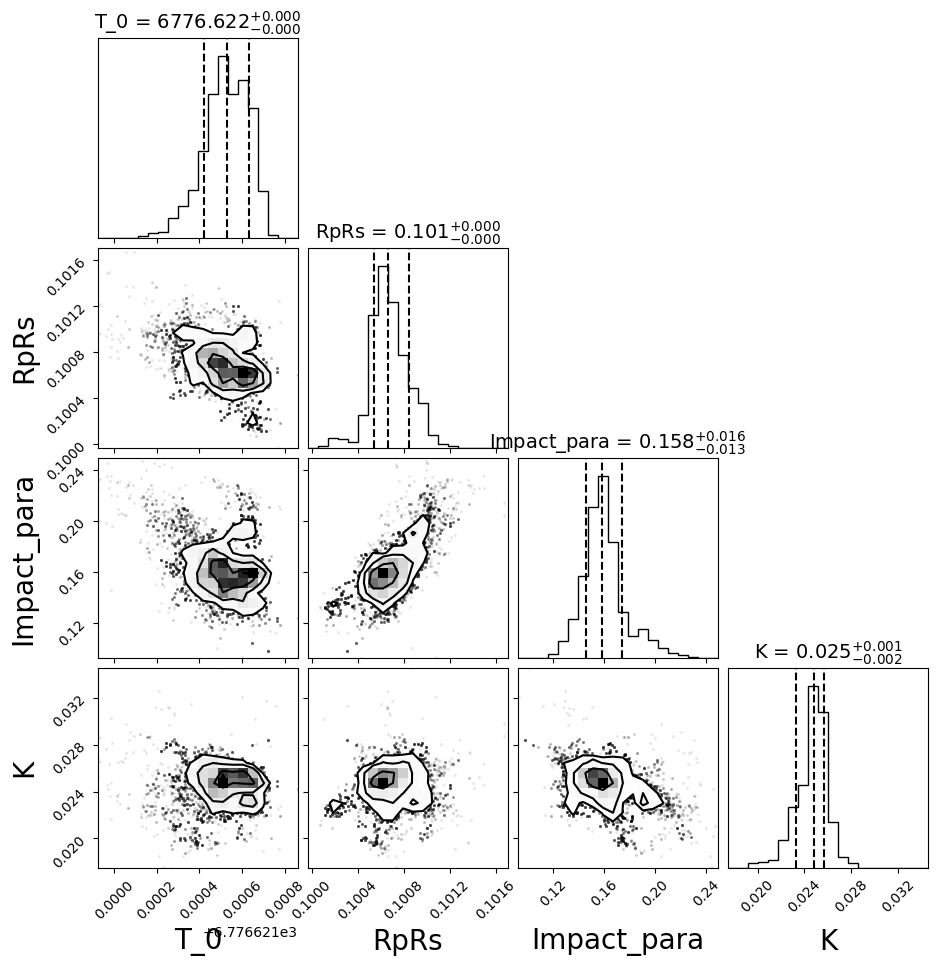
[7]:
%matplotlib inline
[10]:
fig = result.plot_corner(pars = ['T_0', 'RpRs', 'Impact_para', 'K']);
Make customised plots from results#
[11]:
result.lc.names
[11]:
['lc6bjd.dat', 'WASP-127_S9.dat']
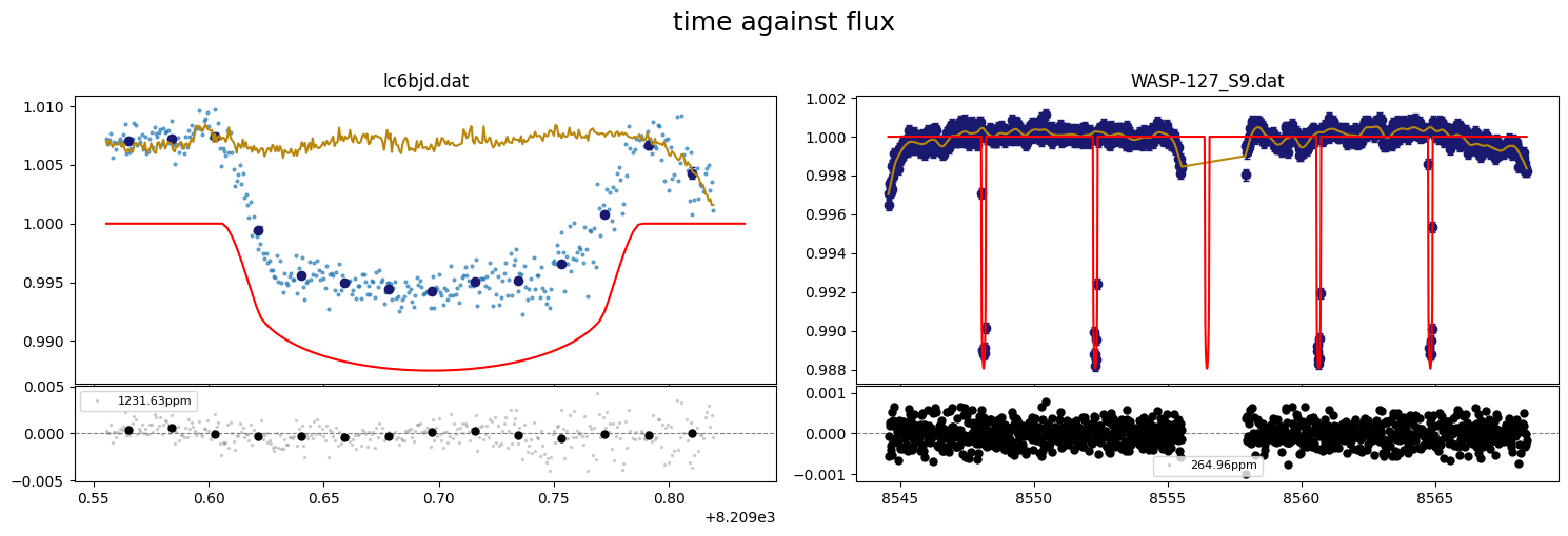
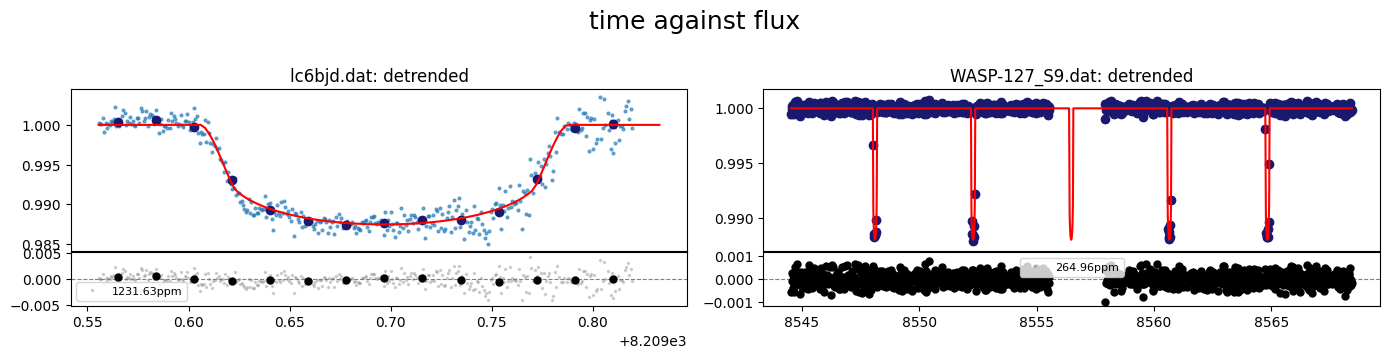
[40]:
fig = result.lc.plot_bestfit(figsize=(15,5))
[52]:
# fig.supxlabel("Time [BJD - 2450000]", x=0.5,y=-0.01)
# fig.axes[0].set_ylabel("Relative flux",fontsize=14)
# fig.axes[1].set_ylabel("O - C", fontsize=14)
# fig.suptitle("")
# fig.savefig("../../../joss/wasp-127.png", dpi=300, bbox_inches='tight')
# fig
[14]:
fig = result.lc.plot_bestfit(detrend=True)
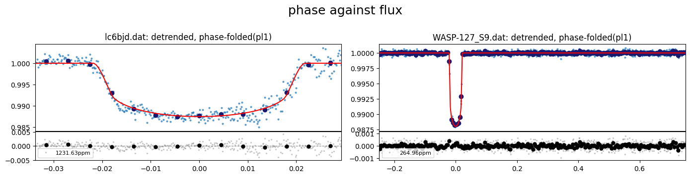
[15]:
# Plot the best fit with phase folding with period of planet 1
fig = result.lc.plot_bestfit(detrend=True, phase_plot=1)
[16]:
#load output data files for the lc fits
lc1data = result.lc.outdata['lc6bjd.dat']
lc2data = result.lc.outdata['WASP-127_S9.dat']

lc1data.keys()
[16]:
Index(['time', 'flux', 'error', 'full_mod', 'base_para', 'base_sine',
       'base_spl', 'base_gp', 'base_total', 'transit', 'det_flux', 'residual',
       'phase'],
      dtype='object')
[17]:
#evaluate LC model on a smoother time array
t_sm  = np.linspace(lc1data["time"].min(), lc1data["time"].max(), 1000)
lcmod = result.lc.evaluate(file="lc6bjd.dat",time=t_sm,return_std = True)

phases = phase_fold(t=t_sm, per=result.params.P, t0=result.params.T0, phase0=-0.5)

#sort
srt    = np.argsort(phases)
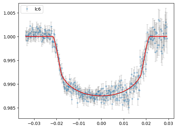
[18]:
plt.errorbar(lc1data["phase"],lc1data["det_flux"],lc1data["error"],
                fmt="o",ms=3,ecolor="gray",alpha=0.3,capsize=2,label="lc6")

plt.plot(phases[srt], lcmod.planet_model[srt],"r",zorder=4)
plt.fill_between(phases[srt],lcmod.sigma_low[srt], lcmod.sigma_high[srt], color="cyan",zorder=3)

plt.legend()
[18]:
<matplotlib.legend.Legend at 0x149cce650>
[19]:
#evaluate LC model on a smoother time array
t_sm   = np.linspace(lc2data["time"].min(), lc2data["time"].max(), 1000)
lc2mod = result.lc.evaluate(file='WASP-127_S9.dat',time=t_sm,return_std=True)

phases = phase_fold(t=t_sm, per=result.params.P, t0=result.params.T0, phase0=-0.5)
#sort
srt    = np.argsort(phases)
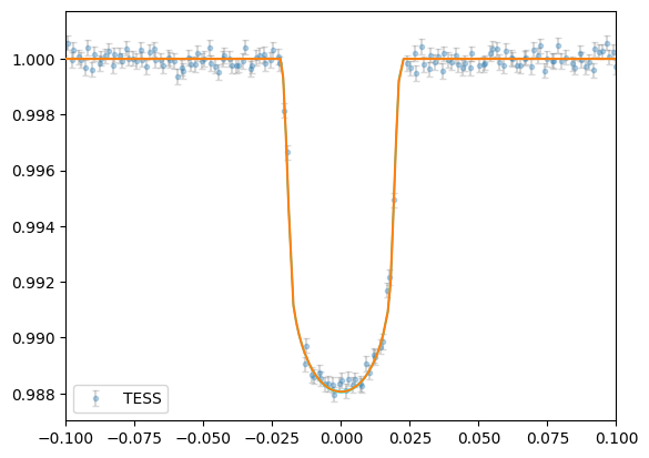
[20]:
plt.errorbar(lc2data["phase"],lc2data["det_flux"],lc2data["error"],
             fmt="o",ms=3,ecolor="gray",alpha=0.3,capsize=2,label="TESS")

plt.plot(phases[srt], lc2mod.planet_model[srt],zorder=4)
plt.fill_between(phases[srt],lc2mod.sigma_low[srt], lc2mod.sigma_high[srt], color="cyan",zorder=3)

plt.xlim([-0.1,0.1])

plt.legend()
[20]:
<matplotlib.legend.Legend at 0x1489e2470>
[21]:
result.rv.names
[21]:
['rv1.dat', 'rv2.dat']
[22]:
%matplotlib inline
[34]:
fig = result.rv.plot_bestfit((0,1,2))
[35]:
fig = result.rv.plot_bestfit((0,1,2),detrend=True)
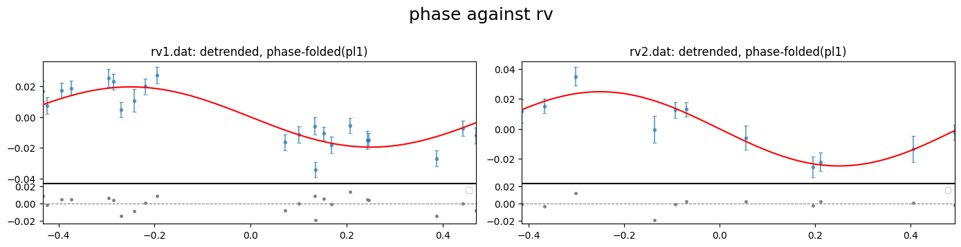
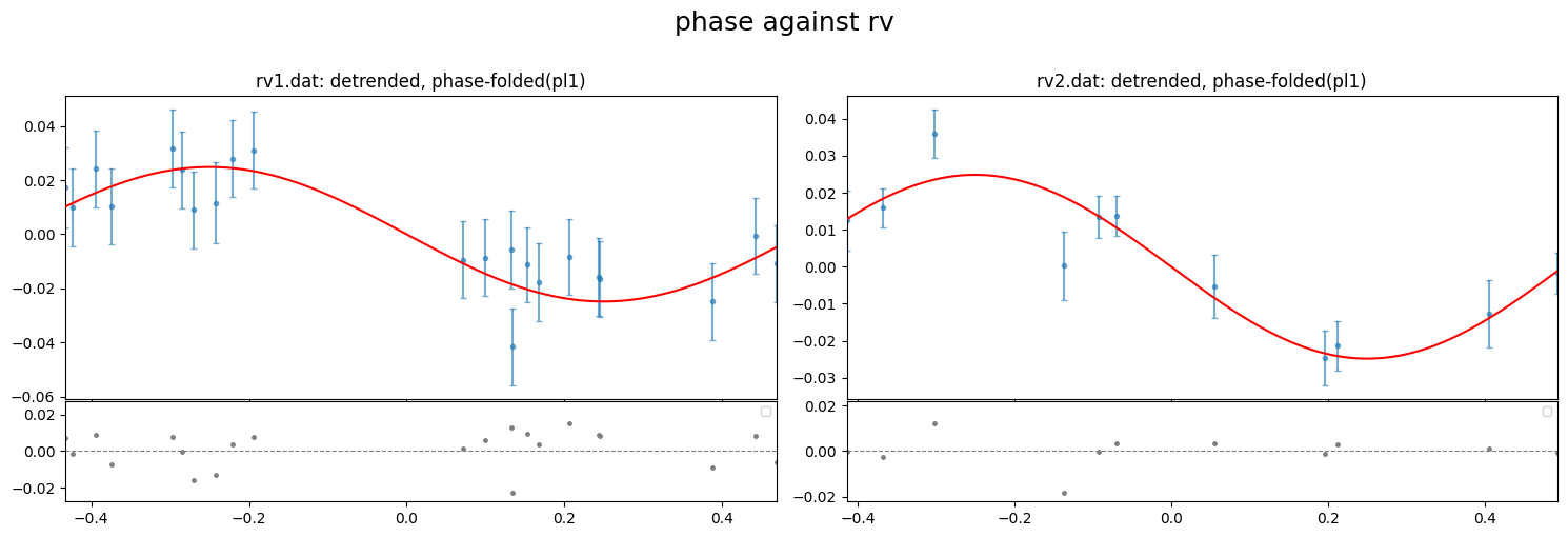
[47]:
fig = result.rv.plot_bestfit((0,1,2), detrend=True, phase_plot=1, figsize=(15,5))
[53]:
# #plot for paper
# fig.supxlabel("Phase", x=0.5,y=-0.005)
# # fig.supylabel("RV [km/s]", y=0.5, x=-0.005)
# fig.axes[0].set_ylabel("RV [km/s]", fontsize=14)
# fig.axes[1].set_ylabel("O - C", fontsize=14)
# fig.suptitle("", fontsize=16)
# # for i in range(len(fig.axes)):
# #     fig.axes[i].set_title(fig.axes[i].get_title().replace("detrended, ",""))
# fig.savefig("../../../joss/wasp-127rv.png", dpi=300, bbox_inches='tight')
# # fig
[49]:
#load output data files for the rv fits
rv1data = result.rv.outdata['rv1.dat']
rv2data = result.rv.outdata['rv2.dat']

rv1data.keys()
[49]:
Index(['time', 'RV', 'error', 'full_mod', 'base_para', 'base_spl', 'base_gp',
       'base_total', 'Rvmodel', 'det_RV', 'gamma', 'residual', 'phase'],
      dtype='object')
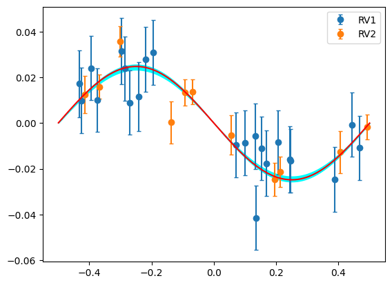
[50]:
#evaluate RV model on a smoother time array
t_sm  = np.linspace(rv1data["time"].min(), rv1data["time"].max(), 1000)
rvmod = result.rv.evaluate(file="rv1.dat",time=t_sm, return_std=True)

phases = phase_fold(t=t_sm, per=result.params.P, t0=result.params.T0, phase0=-0.5)
#sort
srt    = np.argsort(phases)
[51]:
plt.errorbar(rv1data["phase"],rv1data["det_RV"],rv1data["error"],fmt="o",capsize=2,label="RV1")
plt.errorbar(rv2data["phase"],rv2data["det_RV"],rv2data["error"],fmt="o",capsize=2,label="RV2")

plt.plot(phases[srt], rvmod.planet_model[srt],"r",zorder=5)

plt.fill_between(phases[srt],rvmod.sigma_low[srt], rvmod.sigma_high[srt], color="cyan")


plt.legend()
[51]:
<matplotlib.legend.Legend at 0x14dd1c670>
[ ]: