TOI-216: Two-planet TTV fit#
[1]:
from CONAN.get_files import get_TESS_data, get_parameters
import numpy as np
import matplotlib.pyplot as plt
import CONAN
CONAN.__version__
[1]:
'3.3.11'
We will analyse the TESS data of TOI-216 as published in Kipping et. al 2019.
Data download#
[2]:
df = get_TESS_data("TOI-216")
df.search(sectors=[1,2,3,4,5,6], author="SPOC")
SearchResult containing 6 data products.

 #     mission     year author exptime target_name distance
                                  s                 arcsec
--- -------------- ---- ------ ------- ----------- --------
  0 TESS Sector 01 2018   SPOC     120    55652896      0.0
  1 TESS Sector 02 2018   SPOC     120    55652896      0.0
  2 TESS Sector 03 2018   SPOC     120    55652896      0.0
  3 TESS Sector 04 2018   SPOC     120    55652896      0.0
  4 TESS Sector 05 2018   SPOC     120    55652896      0.0
  5 TESS Sector 06 2018   SPOC     120    55652896      0.0
[ ]:
df.download(sectors=[1,2,3,4,5,6],author="SPOC", select_flux="pdcsap_flux",
            quality_bitmask='hardest')

# df.scatter()
[ ]:
df.save_CONAN_lcfile(bjd_ref = 2457000, folder="data")
saved file as: TOI-216/TOI-216_S1.dat
saved file as: TOI-216/TOI-216_S2.dat
saved file as: TOI-216/TOI-216_S3.dat
saved file as: TOI-216/TOI-216_S4.dat
saved file as: TOI-216/TOI-216_S5.dat
saved file as: TOI-216/TOI-216_S6.dat
Data Analysis#
[3]:
from glob import glob
from os.path import basename
lcs = glob("data/TOI*")
lc_list = [basename(lc) for lc in lcs]
lc_list
[3]:
['TOI-216_S1.dat',
 'TOI-216_S2.dat',
 'TOI-216_S3.dat',
 'TOI-216_S6.dat',
 'TOI-216_S4.dat',
 'TOI-216_S5.dat']
[4]:
lc_obj = CONAN.load_lightcurves(   file_list     = lc_list,
                                    data_filepath = "data/",
                                    nplanet       = 2)
lc_obj
# ============ Input lightcurves, filters baseline function =======================================================
name           flt 𝜆_𝜇m |Ssmp ClipOutliers scl_col |off col0 col3 col4 col5 col6 col7 col8|sin id GP spline
TOI-216_S1.dat V   0.6  |None None         None    |  y    0    0    0    0    0    0    0|n    1 n  None
TOI-216_S2.dat V   0.6  |None None         None    |  y    0    0    0    0    0    0    0|n    2 n  None
TOI-216_S3.dat V   0.6  |None None         None    |  y    0    0    0    0    0    0    0|n    3 n  None
TOI-216_S6.dat V   0.6  |None None         None    |  y    0    0    0    0    0    0    0|n    4 n  None
TOI-216_S4.dat V   0.6  |None None         None    |  y    0    0    0    0    0    0    0|n    5 n  None
TOI-216_S5.dat V   0.6  |None None         None    |  y    0    0    0    0    0    0    0|n    6 n  None
[4]:
lightcurves from filepath: data/
2 transiting planet(s)
Order of unique filters: ['V']
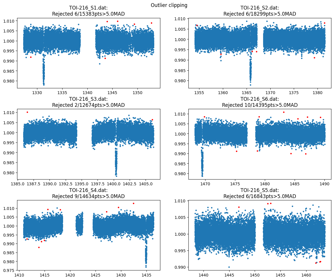
[5]:
lc_obj.clip_outliers(niter=3,show_plot=True)
For multiplanet system, the transit model has to be parameterized by rho_star to reduce the number of free paramters (as opposed to fitting Duration for each planet’s transit)
For TTV fit, we need to fix T_0 and Period for the planets
[6]:
lc_obj.planet_parameters(rho_star    = (2.38, 0.1),
                         RpRs        = [(0.05,0.1,0.15),    #planet b
                                        (0.05,0.1,0.15)],   #planet c
                         Period      = [17.089,             #planet b
                                        34.556],            #planet c
                         T_0         = [1342.42819461 ,     #planet b
                                        1331.28531],        #planet c
                         Impact_para = [(0.5,0.948,1.2),    #planet b
                                        (0,0.15,0.5)]       #planet c
                        )

lc_obj.limb_darkening(  q1  =   (0,0.44,1),
                        q2  =   (0,0.24,1)
                    )
# ============ Planet parameters (Transit and RV) setup ==========================================================
name                       fit  prior                                   note
[rho_star]/Duration        y    N(2.38,0.1)                             #choice in []|unit(gcm^-3/days)
--------repeat this line & params below for multisystem, adding '_planet_number' to the names e.g RpRs_1 for planet 1, ...
RpRs_1                     y    U(0.05,0.1,0.15)                        #range[-0.5,0.5]
Impact_para_1              y    U(0.5,0.948,1.2)                        #range[0,2]
T_0_1                      n    F(1342.42819461)                        #unit(days)
Period_1                   n    F(17.089)                               #range[0,inf]days
[Eccentricity_1]/sesinw_1  n    F(0)                                    #choice in []|range[0,1]/range[-1,1]
[omega_1]/secosw_1         n    F(90)                                   #choice in []|range[0,360]deg/range[-1,1]
K_1                        n    F(0)                                    #unit(same as RVdata)
------------
RpRs_2                     y    U(0.05,0.1,0.15)                        #range[-0.5,0.5]
Impact_para_2              y    U(0,0.15,0.5)                           #range[0,2]
T_0_2                      n    F(1331.28531)                           #unit(days)
Period_2                   n    F(34.556)                               #range[0,inf]days
[Eccentricity_2]/sesinw_2  n    F(0)                                    #choice in []|range[0,1]/range[-1,1]
[omega_2]/secosw_2         n    F(90)                                   #choice in []|range[0,360]deg/range[-1,1]
K_2                        n    F(0)                                    #unit(same as RVdata)
# ============ Limb darkening setup =============================================================================
filters fit     q1                      q2
V       y       U(0,0.44,1)             U(0,0.24,1)
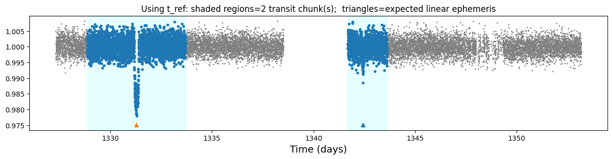
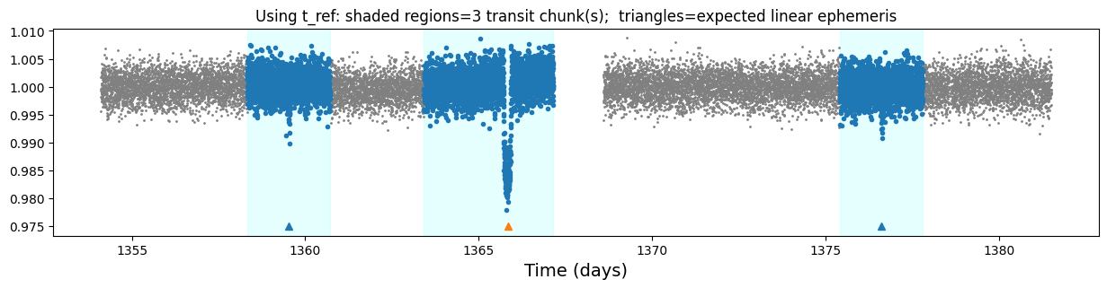
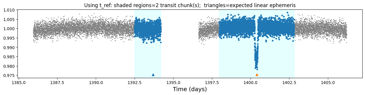
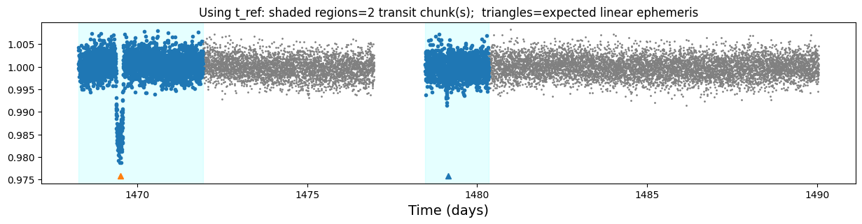
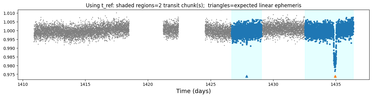
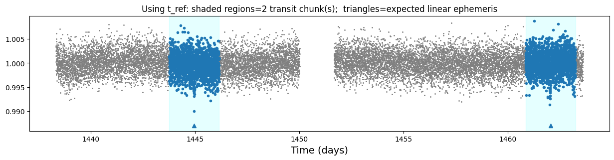
calling the .transit_timing_variation() function with ttvs='y' uses the T_0 and Period values set in .planet_parameters() to search for transits in the data assuming a linear ephemeris.
The print_linear_eph and show_plot arguments provides a print out and plot of the identified linear ephemeris transit times. The shaded region in the plot is the baseline_amount around each identified transit.
dt is the prior that defines the extent of deviation from linear ephemeris for each transit. Default is U(-0.1,0,0.1) indicating a uniform prior ranging between 2.4hrs before and after the expected linear ephemeris transit. N(0,0.1) is a normal prior around the expected transit time
[7]:
lc_obj.transit_timing_variation(ttvs            = "y",
                                dt              = (-0.1, 0, 0.1),
                                baseline_amount = 0.07,
                                show_plot       = True,
                                print_linear_eph= True)
# ============ TTV setup ========================================================================================
Fit_TTVs        dt_priors(deviation from linear T0)     transit_baseline[P]     per_LC_T0       include_partial
y               U(-0.1,0,0.1)                                        0.0700     False           True

======(linear ephemeris estimate)===============
label                   T0s (ordered)           T0s priors
ttv00-lc1-T0_pl2        1331.28531000   U(1331.1853,1331.2853,1331.3853)
ttv01-lc1-T0_pl1        1342.42819461   U(1342.3282,1342.4282,1342.5282)
ttv02-lc2-T0_pl1        1359.51719461   U(1359.4172,1359.5172,1359.6172)
ttv03-lc2-T0_pl2        1365.84131000   U(1365.7413,1365.8413,1365.9413)
ttv04-lc2-T0_pl1        1376.60619461   U(1376.5062,1376.6062,1376.7062)
ttv05-lc3-T0_pl1        1393.69519461   U(1393.5952,1393.6952,1393.7952)
ttv06-lc3-T0_pl2        1400.39731000   U(1400.2973,1400.3973,1400.4973)
ttv07-lc4-T0_pl2        1469.50931000   U(1469.4093,1469.5093,1469.6093)
ttv08-lc4-T0_pl1        1479.14019461   U(1479.0402,1479.1402,1479.2402)
ttv09-lc5-T0_pl1        1427.87319461   U(1427.7732,1427.8732,1427.9732)
ttv10-lc5-T0_pl2        1434.95331000   U(1434.8533,1434.9533,1435.0533)
ttv11-lc6-T0_pl1        1444.96219461   U(1444.8622,1444.9622,1445.0622)
ttv12-lc6-T0_pl1        1462.05119461   U(1461.9512,1462.0512,1462.1512)
model the trend in the data using a GP
[8]:
lc_obj.add_GP(  lc_list     = "same",
                par         = "col0",
                kernel      = 'mat32',
                amplitude   = (1,2000,4000),  #in ppm
                lengthscale = (0.1,1,30),     #in days
                gp_pck      = "ce"
                )
# ============ Input lightcurves, filters baseline function =======================================================
name           flt 𝜆_𝜇m |Ssmp ClipOutliers scl_col |off col0 col3 col4 col5 col6 col7 col8|sin id GP spline
TOI-216_S1.dat V   0.6  |None c1:W15C5n3   None    |  n    0    0    0    0    0    0    0|n    1 ce None
TOI-216_S2.dat V   0.6  |None c1:W15C5n3   None    |  n    0    0    0    0    0    0    0|n    2 ce None
TOI-216_S3.dat V   0.6  |None c1:W15C5n3   None    |  n    0    0    0    0    0    0    0|n    3 ce None
TOI-216_S6.dat V   0.6  |None c1:W15C5n3   None    |  n    0    0    0    0    0    0    0|n    4 ce None
TOI-216_S4.dat V   0.6  |None c1:W15C5n3   None    |  n    0    0    0    0    0    0    0|n    5 ce None
TOI-216_S5.dat V   0.6  |None c1:W15C5n3   None    |  n    0    0    0    0    0    0    0|n    6 ce None
# ============ Photometry GP properties (start newline with name of * or + to Xply or add a 2nd gp to last file) =========
name/filt      kern  par    h1:[Amp_ppm]       h2:[len_scale1]    h3:[Q,η,α,b]       h4:[P]
same           mat32 col0   LU(1,2000,4000)    LU(0.1,1,30)       None               None
detrending the data with a GP automatically sets offset = n to avoid correlations with the GP parameters. we can choose here to set it back to “y” for all lcs.
[9]:
lc_obj._fit_offset = ["y"]*lc_obj._nphot
[10]:
fit_obj = CONAN.fit_setup(apply_LCjitter="y")
fit_obj.sampling(n_cpus=10,n_live=150)
# ============ Stellar input properties ======================================================================
# parameter     value
Radius_[Rsun]  N(1,None)
Mass_[Msun]    N(None,None)
Input_method:[R+rho(Rrho), M+rho(Mrho)]: Rrho
# ============ FIT setup =====================================================================================
Number_steps                              2000
Number_chains                             64
Number_of_processes                       10
Burnin_length                             500
n_live                                    150
force_nlive                               False
d_logz                                    0.1
Sampler(emcee/dynesty)                    dynesty
emcee_move(stretch/demc/snooker)          stretch
nested_sampling(static/dynamic[pfrac])    static
leastsq_for_basepar(y/n)                  n
apply_LCjitter(y/n,list)                  y
apply_RVjitter(y/n,list)                  y
LCjitter_loglims(auto/[lo,hi])            auto
RVjitter_lims(auto/[lo,hi])               auto
LCbasecoeff_lims(auto/[lo,hi])            auto
RVbasecoeff_lims(auto/[lo,hi])            auto
Light_Travel_Time_correction(y/n)         n
save config file#
[ ]:
CONAN.create_configfile(lc_obj=lc_obj, rv_obj=None, fit_obj=fit_obj,
                            filename='TOI216_ttvconfig.dat')
if config file already saved, the entire setup in the previous cells can be loaded with the following command
[12]:
import CONAN
lc_obj, rv_obj, fit_obj = CONAN.load_configfile('TOI216_ttvconfig.dat')

#remember to put back the offsets if required
lc_obj._fit_offset = ["y"]*lc_obj._nphot
Sampling#
[ ]:
result = CONAN.run_fit(lc_obj      = lc_obj,
                        rv_obj      = None,
                        fit_obj     = fit_obj,
                        out_folder  = "result_TOI216",
                        rerun_result= True)
Load result of a previous run#
[14]:
import CONAN
import matplotlib.pyplot as plt
import numpy as np
result = CONAN.load_result("result_TOI216")
['lc'] Output files, ['TOI-216_S1_lcout.dat', 'TOI-216_S2_lcout.dat', 'TOI-216_S3_lcout.dat', 'TOI-216_S4_lcout.dat', 'TOI-216_S5_lcout.dat', 'TOI-216_S6_lcout.dat'], loaded into result object
['rv'] Output files, [], loaded into result object
[16]:
result.lc.plot_lcttv();
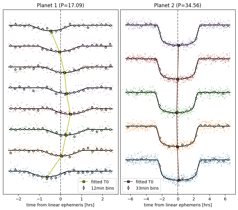
[17]:
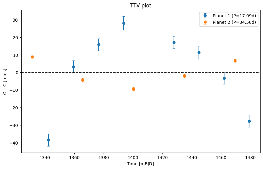
result.lc.plot_ttv();
[18]:
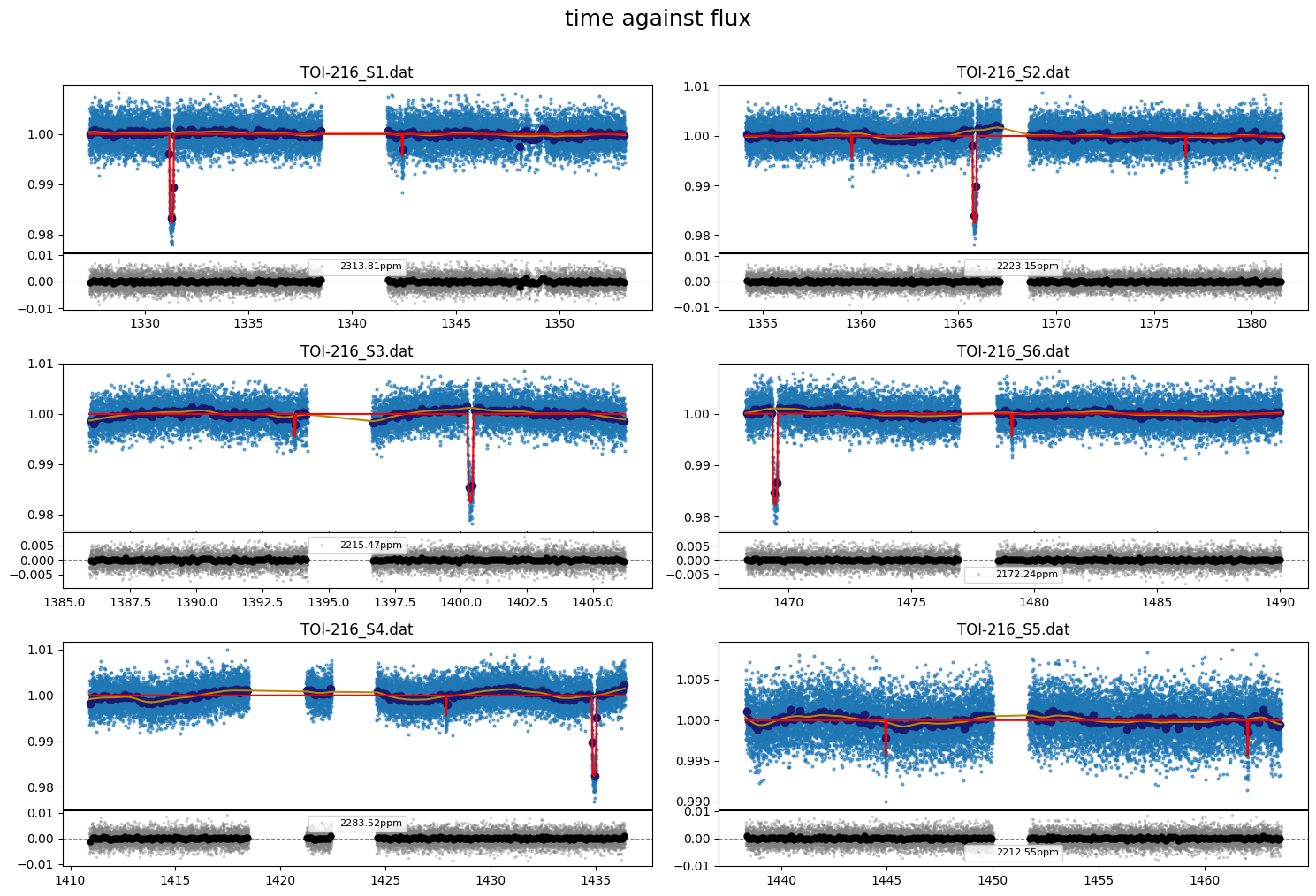
result.lc.plot_bestfit(figsize=(15,10),binsize=0.1);
[19]:
# all varying parameters from the fit
params_dict = result.params_dict
[20]:
#extract all ttv values
{k:v for k,v in params_dict.items() if f'ttv' in k}
[20]:
{'ttv00-lc1-T0_pl2': 1331.2853585351754+/-0.000708561902342808,
 'ttv01-lc1-T0_pl1': 1342.4281946095093+/-0.0024361019883372137,
 'ttv02-lc2-T0_pl1': 1359.5394262797838+/-0.0024319350051200672,
 'ttv03-lc2-T0_pl2': 1365.824496367836+/-0.0007073555550505262,
 'ttv04-lc2-T0_pl1': 1376.630536387638+/-0.002353434384758657,
 'ttv05-lc3-T0_pl1': 1393.7214028843155+/-0.002681758582752991,
 'ttv06-lc3-T0_pl2': 1400.3692862108767+/-0.0006903885439442092,
 'ttv07-lc4-T0_pl2': 1469.4769257299806+/-0.0006485664398496738,
 'ttv08-lc4-T0_pl1': 1479.094324828132+/-0.002385498113653739,
 'ttv09-lc5-T0_pl1': 1427.8784160519003+/-0.002466846340325901,
 'ttv10-lc5-T0_pl2': 1434.9226946540493+/-0.000681746821555862,
 'ttv11-lc6-T0_pl1': 1444.9567796400843+/-0.002506038005321898,
 'ttv12-lc6-T0_pl1': 1462.029002832283+/-0.0024252965312143715}
[21]:
#names of all transit time parameters
import numpy as np
all_T0_names = [nm for nm in result.params.names if 'ttv' in nm]
print(np.array(all_T0_names))
['ttv00-lc1-T0_pl2' 'ttv01-lc1-T0_pl1' 'ttv02-lc2-T0_pl1'
 'ttv03-lc2-T0_pl2' 'ttv04-lc2-T0_pl1' 'ttv05-lc3-T0_pl1'
 'ttv06-lc3-T0_pl2' 'ttv07-lc4-T0_pl2' 'ttv08-lc4-T0_pl1'
 'ttv09-lc5-T0_pl1' 'ttv10-lc5-T0_pl2' 'ttv11-lc6-T0_pl1'
 'ttv12-lc6-T0_pl1']
[ ]:
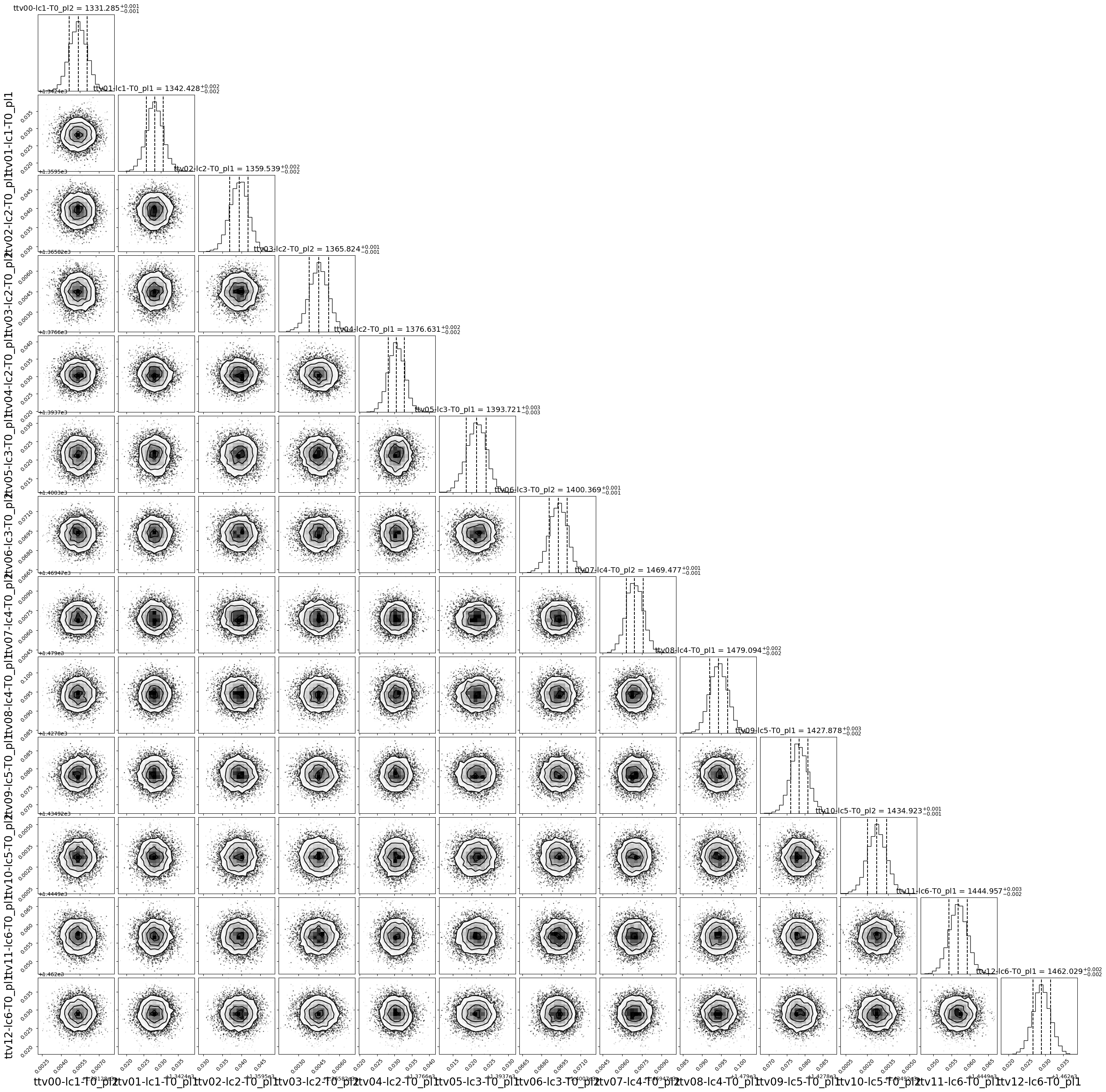
#cornerplot of T0s
fig = result.plot_corner(pars = all_T0_names);
[32]:
#extract ttv values for planet 1

{k:v for k,v in params_dict.items() if f'T0_pl1' in k}
[32]:
{'ttv01-lc1-T0_pl1': 1342.4281946095093+/-0.0024361019883372137,
 'ttv02-lc2-T0_pl1': 1359.5394262797838+/-0.0024319350051200672,
 'ttv04-lc2-T0_pl1': 1376.630536387638+/-0.002353434384758657,
 'ttv05-lc3-T0_pl1': 1393.7214028843155+/-0.002681758582752991,
 'ttv08-lc4-T0_pl1': 1479.094324828132+/-0.002385498113653739,
 'ttv09-lc5-T0_pl1': 1427.8784160519003+/-0.002466846340325901,
 'ttv11-lc6-T0_pl1': 1444.9567796400843+/-0.002506038005321898,
 'ttv12-lc6-T0_pl1': 1462.029002832283+/-0.0024252965312143715}
[ ]: